specINTI & specINTI Editor
Appendix 4: Questions and Answers
This part gathers a small library of configuration files and tips for using specINTI covering various operating modes. These are answers to questions you may have about the use of the software. You can pick up ideas adapted to your current configuration and of course, copy and paste YAML files. It is also an opportunity to present some "non-standard" ways of using the software. This part is also a guide to the good use of a spectrograph, in particular Star'Ex.
A4.1 : I have to process spectra with medium spectral resolution captured with a relatively small telescope, how to do it ?
The term medium spectral resolution applies to spectra with a resolving power R of between 1500 and 8000, i.e. a spectral sharpness of between 3.5 and 0.7 angstroms.
Let's take the example of the Star'Ex spectrograph, which offers great flexibility of use. It can be configured in a "low resolution" mode, i.e. Star'Ex LR ("Low Resolution", 80x80 optical arrangement, 300 t/mm grating), or in a "high resolution" mode, i.e. Star'Ex HR ("High Resolution", 80x125 configuration, 2400 t/mm grating, a base very close to the Sol'Ex instrument).
Intermediate arrangements are possible, for example in the situation described here, an 80x125 mm configuration, but with a grating of 600 lines/mm. The goal is to reduce the spectral dispersion, compared to a grating of 2400 lines/mm in order to cover a spectral range from the red line of helium at 6678 A, to the yellow line of helium at 5875 A (important note for the users of Star'Ex : one could imagine using an 80x80 configuration here with a 1200 t/mm grating, but the idea is not a good one because the 80 mm camera lens is specifically optimized for use with a 300 t/mm grating, and gives spectrum images that may prove disappointing with other etch densities).
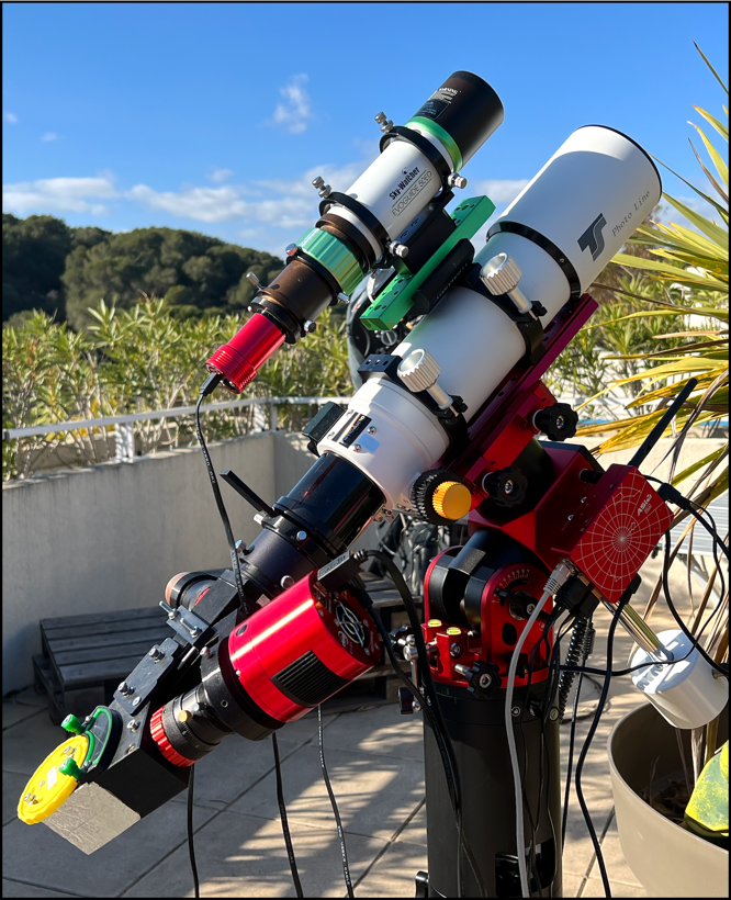
Star'Ex is here mounted on the back of a so-called "APO" refractor, 80 mm in diameter and 480 mm in focal length, i.e. an F/D ratio of 6. This is the TS PhotoLine 80 mm model. With such a focal length, a slit of 15 microns wide is appropriate, covering 6.5 arcseconds on the sky (a slit of 10 microns is also compatible, giving even a higher spectral resolution power, but although this is not absolutely prohibitive, we are wary here of atmospheric chromatism and of the telescope, which can induce sensitive spectrophotometric biases with such a narrow slit). In this case, the quantity of flux entering the spectrograph is favored at the cost of a slight loss of spectral resolution. The power of resolution reached is about R = 2400. The camera is a ZWO ASI533MM.
Here is the aspect of the raw image of the spectrum of the star AX Per (a symbiotic star of magnitude 10.6) obtained after an exposure of 600 s performed with this equipment (in urban conditions):
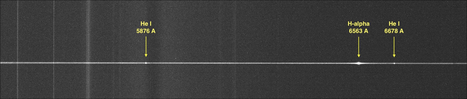
The spectrum turns out to be very fine. In addition to the quality of the spectrograph, we must mention the relatively large size of the pixels of the camera used, 3.75 microns, which will not fail to pose a problem because of the potential undersampling that this induces, as we will see.
How to calibrate such a spectrum in wavelength? This is often the tricky question. Here we went to the simplest: a neon bulb (or night light) powered by 220 V, as described in part 5 of this documentation (never directly on the 220 V mains), that we shake in front of the 80 mm diameter of the telescope by interposing a sheet of tracing paper to obtain a uniform illumination. It is a quick technique that can be described as manual, but nevertheless effective. The image below is made under these conditions in 30 seconds:
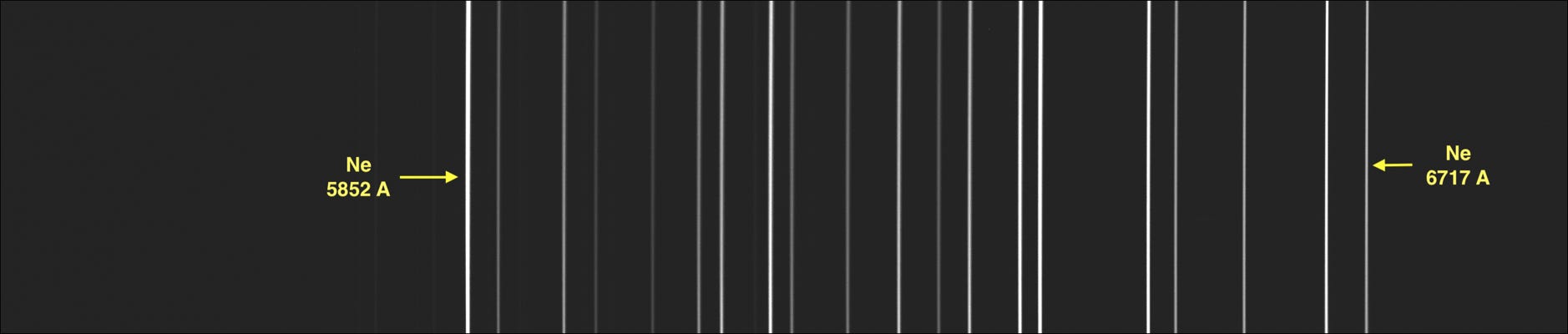
We note that the spectral range is well covered by the standard lines, with a uniform distribution, ideal for calibration.
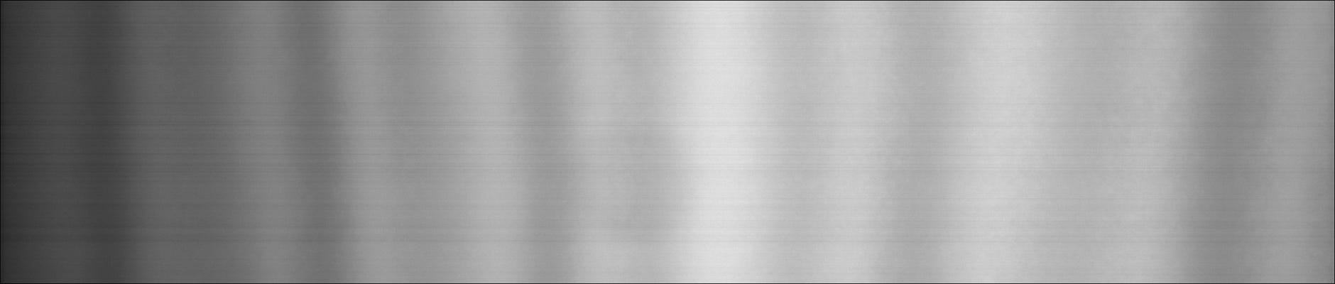
The flat-field is obtained in a very similar way, with a flashlight type "MagLite mini" with xenon bulb in front of the entrance pupil and interposing a sheet of tracing paper. The exposure time is still 30 seconds while the color temperature of the continuous spectrum produced is evaluated at 2700 K (note the spectral ripples, somehow the signature of Sony CMOS sensors):
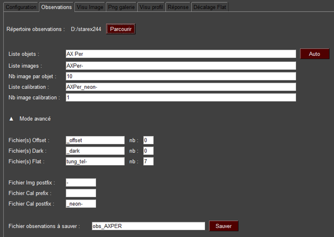
We have realized 10 spectral images of AX Per, each exposed for 600 seconds. The available dataset allows us to write the observation YAML file as follows ("Observations" tab of specINTI):
# ********************************************************************************
# Configuration Star'Ex moyenne resolution (R=2300)
# Réseau 600 t/mm - 80x125 - fente 15 microns
# Lunette TS80 - F=480
# Mode étalonnage 0
# ********************************************************************************
# ---------------------------------------------------
# Répertoire de travail
# ---------------------------------------------------
working_path: D:/starex244
# ---------------------------------------------------
# Fichier batch de traitement
# ---------------------------------------------------
batch_name: obs_AXPER
# ---------------------------------------------------
# Mode d'étalonnage spectral
# ---------------------------------------------------
calib_mode: 0
# ----------------------------------------------------------------------
# Recherche automatique des raies d'étalonnage
# ---------------------------------------------------------------------
auto_calib: [5800, 7100]
# ---------------------------------------------
# Ordre polynôme
# --------------------------------------------
poly_order: 2
# --------------------------------------------
# Largeur de binning
# --------------------------------------------
bin_size: 18
# ---------------------------------------------------
# Zones de calcul du fond de ciel
# ---------------------------------------------------
sky: [150, 20, 20, 150]
# ---------------------------------------------------
# Mode extraction du ciel
# ---------------------------------------------------
sky_mode: 1
# -----------------------------------------------------------------------
# Bornes horizontales pour mesures géométriques
# -----------------------------------------------------------------------
xlimit: [400, 1800]
# ----------------------------------------------------------------
# Largeur en pixels de la zone de recherche des raies
# d'étalonnage spectral
# ----------------------------------------------------------------
search_wide: 40
# -------------------------------------------------------------
# Réponse instrumentale
# ------------------------------------------------------------
instrumental_response: _rep
# ----------------------------------------------------------------
# Température de couleur du tungstène
# ----------------------------------------------------------------
planck: 2700
# ----------------------------------------------------------------
# Motif de filtrage médian
# ----------------------------------------------------------------
kernel_size: -3
# ----------------------------------------------------------------
# Filtrage gaussien
# ----------------------------------------------------------------
sigma_gauss: 0.5
# ----------------------------------------------------------------
# Zone de normalisation à l'unité
# ----------------------------------------------------------------
norm_wave: [6640, 6660]
# ----------------------------------------------------------------
# Zone de cropping du profil
# ----------------------------------------------------------------
crop_wave: [5416, 6860]
# ----------------------------------------------------------------
# Longitude du lieu d'observation
# ----------------------------------------------------------------
Longitude: 7.0940
# ----------------------------------------------------------------
# Latitude du lieu d'observation
# ----------------------------------------------------------------
Latitude: 43.5801
# ----------------------------------------------------------------
# Altitude du lieu d'observation en mètres
# ----------------------------------------------------------------
Altitude: 40
# ----------------------------------------------------------------
# Site d'observation
# ----------------------------------------------------------------
Site: Antibes Saint-Jean
# ----------------------------------------------------------------
# Description de l'instrument
# ----------------------------------------------------------------
Inst: TS80 + StarEx600 + ASI533MM
# ----------------------------------------------------------------
# Observateur
# ----------------------------------------------------------------
Observer: cbuil
# ----------------------------------------------------------------
# Goodies
# ----------------------------------------------------------------
check_mode: 0
The selected calibration mode is number 0, i.e. the most classical mode, consisting in establishing the dispersion polynomial directly from the line spectrum of the calibration lamp distinct from the science images. Here is the corresponding configuration file:
The salient points to note are as follows:
The calculated dispersion polynomial is of degree 2, which is considered sufficient in the circumstances for the spectral region of interest ("poly_order: 2" parameter)
We exploit the automatism offered by specINTI to find the adequate calibration spectral lines ("auto_calib" parameter). Given the spectral range of line search requested, between 5800 A and 7100 A, we include the intense neon line located at 5852 A. In addition to the fact that it is necessary to take care that this line is not saturated in the acquired data, it is important here to use version 2.1 and above of specINTI, which knows how to manage such a difference in the intensity of the calibration lines. But if you absolutely want to avoid this pitfall, then reject the line at 5852 A by writing for example
auto_calib: [5865, 7100]
Note: for information, here is the list of neon lines used by the "auto_calib" parameter:
[5852.488,5881.895,5944.834,5975.534,6029.997, 6074.338, 6096.163,6143.063,6163.594,6217.281,6266.495,6304.789,
6334.428,6382.992,6402.246,6506.528,6532.882,6598.953, 6678.276,6717.043,6929.467, 7032.41,7245.167,7438.891,7488.871]
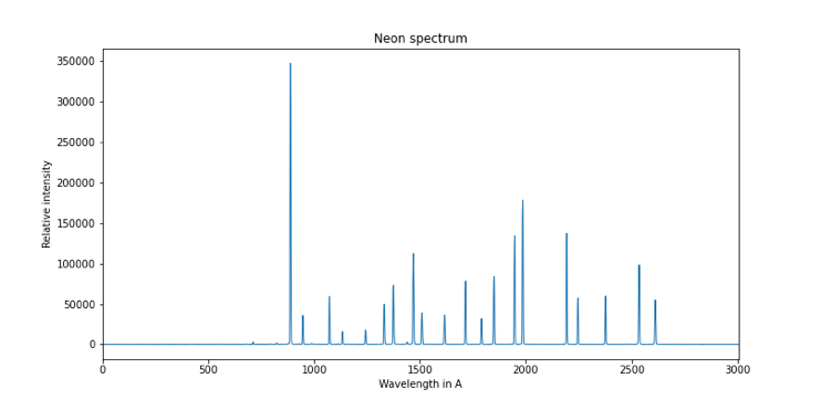
Here is the raw spectral profile of our neon spectrum (it is the profile "profile2.fits", automatically created in your working folder if you give the value 1 to the parameter "check_mode" :
The salient points to note are as follows:
The calculated dispersion polynomial is of degree 2, which is considered sufficient in the circumstances for the spectral region of interest ("poly_order: 2" parameter)
We exploit the automatism offered by specINTI to find the adequate calibration spectral lines ("auto_calib" parameter). Given the spectral range of line search requested, between 5800 A and 7100 A, we include the intense neon line located at 5852 A. In addition to the fact that it is necessary to take care that this line is not saturated in the acquired data, it is important here to use version 2.1 and above of specINTI, which knows how to manage such a difference in the intensity of the calibration lines. But if you absolutely want to avoid this pitfall, then reject the line at 5852 A by writing for example
In the difficult (but very rare) situation of a calibration file strongly disturbed by noise, you have at your disposal a parameter that avoids false line detections. For example, by writing in the configuration file :
auto_calib:_th: 8000
specINTI will only use lines with a peak intensity greater than 8000 ADU. But in general, let the software do it. Here is the result for the example :
Evaluate lines position...
Automatic search of calibration lines...
Number of calibration lines find = 20
$$$$$ -> _step12
5852.488, 5881.895, 5944.834, 5975.534, 6029.997, 6074.338, 6096.163, 6143.063, 6163.594, 6217.281, 6266.495, 6304.789, 6334.428, 6382.992, 6402.246, 6506.528, 6532.882, 6598.953, 6678.276, 6717.043
----------
888.3404699713926, 947.168649886995, 1073.0207351633017, 1134.3070633258953, 1243.2822646234722, 1331.7772667324907, 1375.4297922019791, 1469.222206046395, 1510.1922560569312, 1617.4027624188557, 1715. 653553963965, 1792.086445693, 1851.2337512415368, 1948.1275163464265, 1986.5211525384505, 2194.3757754688095, 2246.8625520071387, 2378.41830399976, 2536.199924474355, 2613.2766976438998
----------
Calibration function...
$$$$$ -> _step13
Calibration coefficients:
8.824634483115597e-07, 0.4980564871959794, 5409.901650996256
O-C: [-0.054 -0.042 -0.009 0.048 0.007 0.071 0.051 0.001 0.019 0.014
0.005 -0.006 -0.016 -0.035 -0.036 -0.044 -0.037 -0.025 0.03 0.058]
Root Mean Square Error = 0.0363 A
The RMS error of calibration is only 0.04 A, which is excellent (but be careful, we only count here the errors related to the noise statistics, not the calibration biases).
Although the spectrum trace is very fine, we allow ourselves to perform a median filtering of the RTS noise by doing :
kernel_size: -3
Here again, version 2.1 and above of specINTI brings an improvement that allows this type of filtering on a poorly sampled spectrum (quasi undersampling here). Be careful with this parameter though, by analyzing the appearance of the spectrum with it and without it.
On the other hand, we avoid here as much as possible to perform an optimal extraction of the spectral profile (Horne's algorithm) by writing something like :
extract_mode: 1
gain: 0.083
noise: 1.3
Indeed, our spectrum is very narrow, which can disturb the algorithm and produce artifacts in the profile (looking like spurious peaks). This quasi undersampling is always a problem (appearance of pseudo noises), so we must be careful. In any case, the primary use of the "extract_mode" parameter set to 1 being the reduction of noise in very low intensity spectra, displaying a signal to noise ratio of 5 to 20 typically to obtain a visible effect, the use of the optimal extraction for our AX Per spectrum, quite intense in the limages, is not justified. So, if you are using a small refractor delivering very narrow spectra (a width at half height of the order of 2 pixels or less), watch carefully the use of the "extract_mode" parameter, and even not secure, do not use it if the spectrum is a bit intense.
A4.2: I have just acquired images of the spectrum of a comet, how to process them?
To answer the question we will set up the configuration file to process a spectrum of comet C/2022 E3 (ZTF), taken on January 31, 2023. We use the same equipment as described in part A4.1 of this appendix (80 mm refractor, Star'Ex equipped with a 600 line/mm array).
We describe only the modifications to be made to the configuration file with respect to the observation of a star.
The first modification concerns the removal of the sky background. During this operation we may not want to remove the emission lines of the coma of the comet, which may extend far from the nucleus. The situation for comet C/2022 E3:
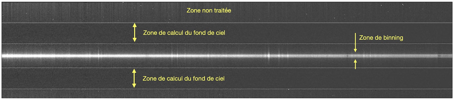
About this image, here is a useful tip. If you write in the configuration file :
check_mode: 1
specINTI generates in the working directory a number of images and intermediate spectral profiles to check the correct operation. Among the image files written in this way, the file "_step101.fits" is surely the most interesting. It is this one which is represented above. It is useful because marks are drawn in this 2D image of the spectrum, which show the limits of the binning zones, the limits of the sky background calculation zones, the vertical position defining the center of the calculated spectrum. You can refer to this image to check the relevance of your settings when setting up the configuration file. For example, you can check that the binning area is sufficiently wide compared to the width of the spectrum trace (push the display contrast). Once the sky background and binning constants are set, you don't have to come back to this image file in principle (but a check from time to time can't hurt).
The sky background calculation areas are here well away from the central area of the spectrum in order to preserve the spectral signature of the coma. For this we do in this example :
sky: [220, 80, 80, 220]
The inner part of the sky background evaluation area is located at 80 pixels from the center of the coma (this is an example, and this choice is more or less arbitrary). We note here that the very good quality of the spectral images along the spatial axis delivered by Star'Ex, an asset for this type of study. In a way, Star'Ex is a wide field spectrograph !
Still in this example, we chose a binning width quite small (18 pixels):
bin_size : 18
The idea is to obtain the spectrum of the near nucleus. But it is perfectly possible to choose a much larger value, 60 pixels for example, to integrate both the spectrum of the nucleus and the coma.
The "posy" parameter in the configuration file may be important. In the example, this parameter is not present in the configuration file because it is considered that the trace of the comet spectrum is sufficiently well marked in the raw images for specINTI to unambiguously identify the vertical coordination (Y) of the trace. But it can happen that the trace is barely perceptible, in this case you have to tell specINTI what is the approximate vertical coordinate of it in pixels-. For example :
posy: 284
In this example, the binning is forced to be done around the Y coordinate = 284 pixels.
In the case of comets, but also nebulae, this ability to manually define the center of the binning area can be used to realize the spectrum of a particular region of the object along the direction of the slit, for example the coma, excluding the core. This procedure is very flexible, but remember to use the file "_step101.fits" to check what you do with the "posy" parameter, and also the calculation areas of the sky background, which follow this coordinate (not necessarily centered)
Remember that a variant of use of "posy" is to provide a negative value, for example :
posy: -284
In this case, specINTI refocuses the traces of the spectra in a sequence, but only in the width of the binning area provided through the "bin_size" parameter. This technique is a powerful way to realize the spectrum of a faint object in an image dominated by the bright trace of a nearby object. It is the "posy" parameter with a negative value that you would use, for example, to extract the spectrum of a supernova in a distant galaxy.
However, in the overwhelming majority of situations, you don't have to set the "posy" parameter: let specINTI do the work of finding the spectra for you, automatically.
Finally, it is not at all recommended, when processing a comet (or nebula) spectrum, to use the optimal spectral profile extraction mode. In these situations, always do :
extract_mode: 0
or delete this parameter if it is present.
On the other hand, you have every right to use the noise reduction tools ("kernel_size" or "sigma_gauss").
A4.3 : Can we use telluric lines to increase the precision of the spectral calibration ?
The telluric lines are produced when the light of the star crosses the terrestrial atmosphere. Thus we find in the visible part, the trace of the lines of water vapor (H2O) or di-oxygen (O2). These lines are most often considered as parasites that interfere with the readability of the spectra (in the infrared, it is bands of lines that can even prevent any observation). But they are also an opportunity when we know how to use them, because they form a set of fine reference lines, with known and precise positions, which can help to better calibrate the spectra.
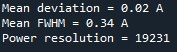
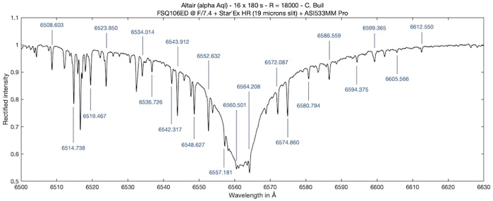
The answer is yes to the question, and particularly at the level of the Halpha line of hydrogen, in the red, when we are interested in high spectral resolution. In this part of the spectrum the H2O lines are numerous, as shown in the following spectrum of the star Altair :
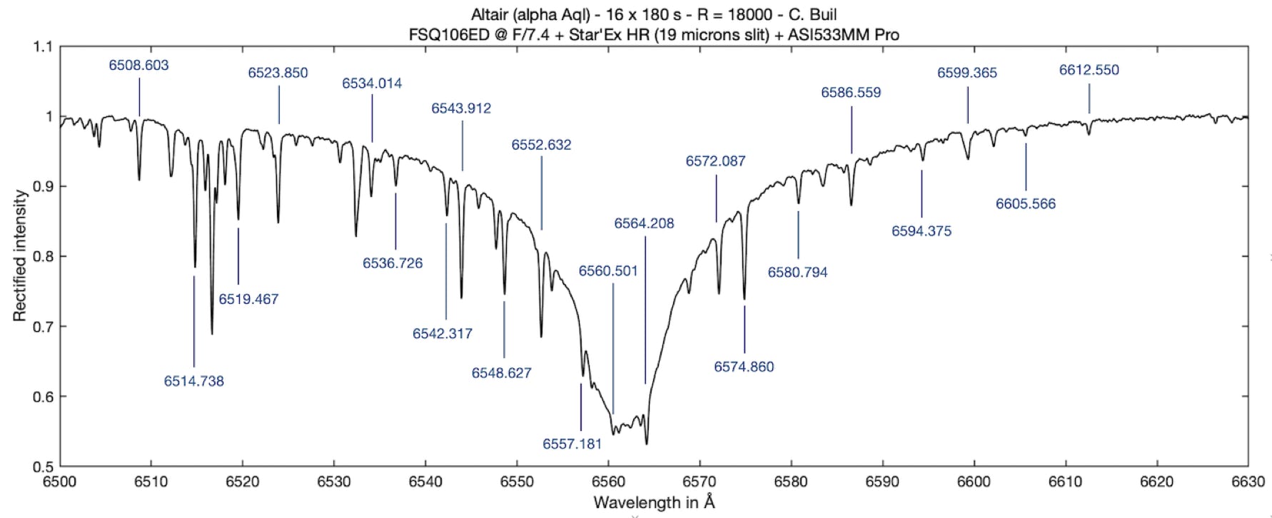
In the spectrum of this hot star, the profile of the Halpha line is very spread out by the high rotation speed of the star on its axis. The wavelength of the telluric lines of water vapor is indicated. These are very fine lines by nature, which can also serve to measure the spectral resolution of the spectrograph.
In this graph, only the wavelengths (in air) of the lines actually usable for calibration are indicated (good contrast, isolated). Here is how to exploit what Nature offers us.
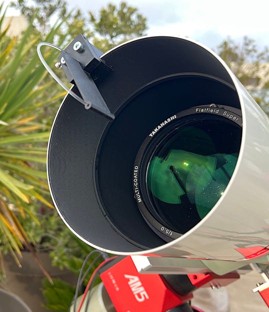
The example taken is that of the double spectroscopic star alpha Draconis. The observation is made with a Star'Ex HR equipped with a 19 microns wide slit and an ASI533MM camera. The image is taken at the focus of a Takahashi FSA106ED refractor of 106 mm diameter and 530 mm focal length at the base. Unfortunately the F/D ratio of 5 of this good telescope (an astrograph in fact) is not compatible with a good use of Star'Ex HR. The high incidence of light rays on the 2400 lines/mm diffraction grating causes a strong optical vignetting when the entrance beam is as open as f/5 (see section A4.7). A Barlow lens is added in front of the slit to bring the focal length to 790 mm, that is to say an F/D of 7.4, much more satisfactory.
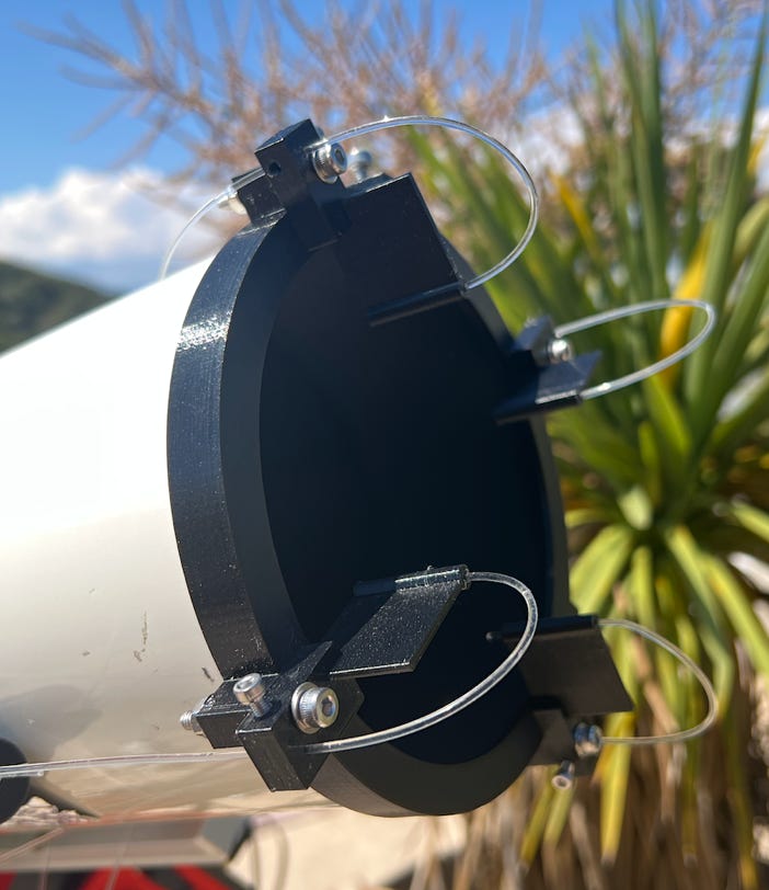
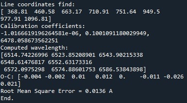
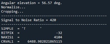
Moreover, the observation is carried out in lateral mode (mode 3), i.e. with a spectral lamp source (here neon) permanently arranged at the entrance of the telescope (and of small surface not to obstruct too much the entrance pupil). In this case, the light is injected at the entrance of the FSQ10E6ED by a cheap plastic optical fiber of 2 mm diameter. This light is permanently on during the taking of spectra (elementary exposures of 600 seconds in this case). You can of course choose an intermittent lighting and any other light source, or use several fibers for a more homogeneous lighting. The result is a composite image of the star spectrum and the calibration lines. Opposite, the injection system of the calibration source at the front of the FSQ106ED (a single fiber in this case).
Hereafter, a raw spectrum of alpha Draconis (600 seconds) with the trace of the spectrum of the star and the lines of the neon in overprint (very fine lines):
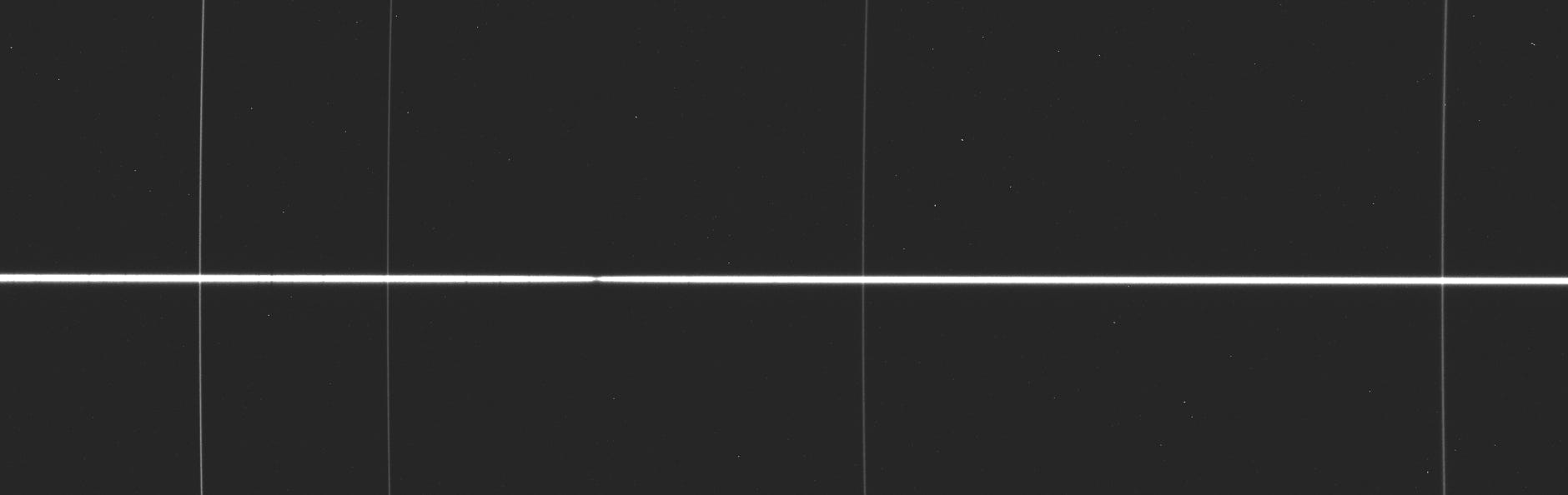
We have a simultaneous shot of the spectrum of the star and the artificial standard source. The gain in calibration accuracy is potentially significant because it erases in this way a large part of the calibration errors associated with variable mechanical bending of the instrument. We do not have to worry about the mixing of these standard lines with the spectrum of the star: the first ones are discrete and if necessary, they can be deleted during processing by writing in the configuration file something like :
clean_wave: [6506.5, 6532.8, 6598.9, 6678.3]
clean_wide: [1.1, 0.8, 0.9, 1.0]
Here is the complete configuration file used to process the alpha Draconis (or other) spectra in high resolution and mode 3 (lateral):
# *******************************************************
# Configuration Star'Ex haute résolution
# Réseau 2400 t/mm - 80x125 - fente 19 microns
# Mode étalonnage 3
# *******************************************************
# ---------------------------------------------------
# Répertoire de travail
# ---------------------------------------------------
working_path: D:/starex287
# ---------------------------------------------------
# Fichier batch de traitement
# ---------------------------------------------------
batch_name: obs_alpha_dra
# ---------------------------------------------------
# Mode d'étalonnage spectral
# ---------------------------------------------------
calib_mode: 3
# ---------------------------------------------
# Recherche automatique des raies d'étalonnage
# ---------------------------------------------
auto_calib: [6490, 6690]
# ---------------------------------------------
# Ordre du polynôme de dispersion spectrale
# --------------------------------------------
poly_order: 2
# --------------------------------------------
# Largeur de binning
# --------------------------------------------
bin_size: 20
# ---------------------------------------------------
# Zones de calcul du fond de ciel
# ---------------------------------------------------
sky: [160, 16, 16, 160]
# --------------------------------------------
# Rayon de smile
# --------------------------------------
smile_radius: -17000
# ---------------------------------------------------
# Mode extraction du ciel
# ---------------------------------------------------
sky_mode: 1
# ---------------------------------------------------
# Domaine de calcul des paramètres géométriques (en pixels)
# ---------------------------------------------------
xlimit: [400, 1800]
# -----------------------------------------------------------
# Incertitude de recherche des raies d’étalonnage (en pixels)
# -----------------------------------------------------------
search_wide: 40
# -------------------------------------------------------------
# Réponse instrumentale
# ------------------------------------------------------------
instrumental_response: _rep
# -----------------------------------------------------------
# Motif de filtrage médian (-3, retrait optimal du bruit RTS)
# -----------------------------------------------------------
kernel_size: -3
# ------------------------------------------------------------
# Filtrage gaussien (passe la résolution de R=24000 à R=19000)
# ------------------------------------------------------------
sigma_gauss: 0.5
# ----------------------------------------------------------------
# Zone de normalisation du continuum à l'unité
# ----------------------------------------------------------------
norm_wave: [6640, 6660]
# ----------------------------------------------------------------
# Zone de cropping du profil
# ----------------------------------------------------------------
crop_wave: [6481, 6695]
# ----------------------------------------------------------------
# Pouvoir de résolution (imposé en mode 3)
# ----------------------------------------------------------------
power_res: 19000
# ----------------------------------------------------------------
# Longitude du lieu d'observation
# ----------------------------------------------------------------
Longitude: 7.0940
# ----------------------------------------------------------------
# Latitude du lieu d'observation
# ----------------------------------------------------------------
Latitude: 43.5801
# ----------------------------------------------------------------
# Altitude du lieu d'observation en mètres
# ----------------------------------------------------------------
Altitude: 40
# ----------------------------------------------------------------
# Site d'observation
# ----------------------------------------------------------------
Site: Antibes Saint-Jean
# ----------------------------------------------------------------
# Description de l'instrument
# ----------------------------------------------------------------
Inst: FSQ106ED + StarEx2400 + ASI533MM
# ----------------------------------------------------------------
# Observateur
# ----------------------------------------------------------------
Observer: cbuil
# ----------------------------------------------------------------
# Goodies
# ----------------------------------------------------------------
check_mode: 0
clean_wave: [6506.5, 6532.8, 6598.9, 6678.3]
clean_wide: [1.1, 0.8, 0.9, 1.0]
simbad: 1
corr_atmo: 0.10
spectral_shift_wave: 0.02
In this listing you should pay attention to the last line:
spectral_shift_wave: 0.02
It means that compared to the spectral calibration calculated automatically by specINTI, a spectral shift of 0.02 A is added to make everything perfect on the side of this calibration. It is not abnormal to have to retouch the calculated calibration, even in lateral mode. The way to illuminate the entrance of the telescope is not the same depending on whether the light comes from the stars or from the standard source (here a point in the pupil). This produces a small bias. It is reduced a little if instead of a single fiber we use several (4 for example).
However, in this example we felt the need to make a slight adjustment of 0.02 A (or about 1 km / s at the Halpha line). This is not negligible when looking for a high accuracy of radial velocity measurement (restitution of the orbit of the alpha Draconis couple), and even if we are very close to the possibilities of Star'Ex in the mode used (0.02 A is 1/18 of times narrower than the most resolvable details in the spectrum!)
The question is: how do we find this value of 0.02 A?
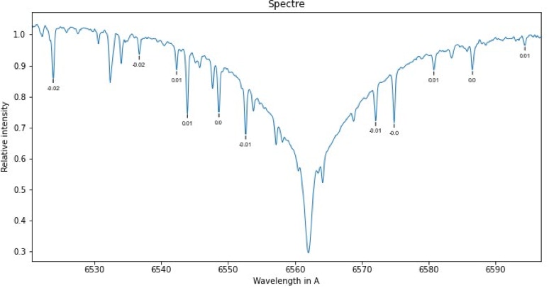
The telluric lines bring the solution, and here is how to exploit them with specINTI and specINTI Editor. Start by performing a normal processing, without spectral shift (the value of "spectral_shift_wave" is 0). Then display the profile found from the tab " Visu profil " of secINTI Editor, then click on the button " Vérif atm ". Here is what we get in the example:
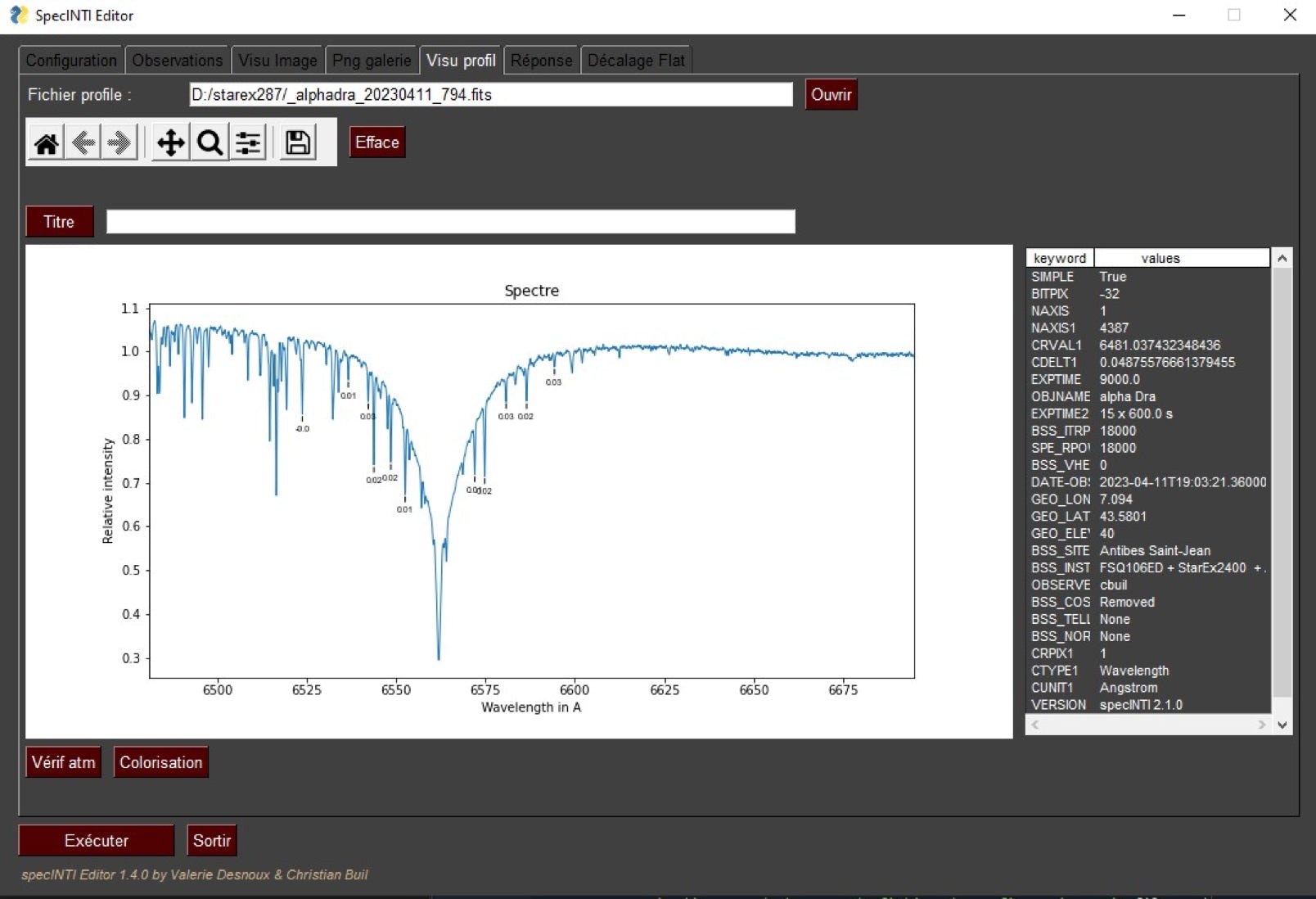
The position of some telluric lines around the Halpha line of the alpha Draconis star are identified by marks, and above all, specINTI Editor has calculated very precisely the difference between the theoretical wavelength (or catalog) of the telluric lines and their measured wavelengths in our spectrum (we proceed by a gaussian adjustment of each telluric line). Let's have a close look at this result (you can enlarge with the magnifying glass of the interface) :
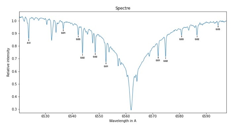
We note that the characteristic offset between the theory and the observed is about +0.02 A. This result is found in the output console of specINTI, in the following form:
As a bonus, the average sharpness of the selected telluric lines has been calculated, and a satisfactory value of the resolving power is returned (here R = 19000).
It is here that we use the "spectral_shift_wave" parameter by assigning it the value +0.02. Let's resume the calculation of the spectrum in this situation, and here is the result on the telluric lines:
The spectral shift is very close to 0 A :
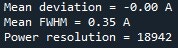
The spectral calibration is satisfactory and the spectrum is good for the service: to calculate the radial velocity of a double spectroscopy, for example to participate in an observing campaign such as STAROS, or to feed a database such as BESS when interested in Be stars.
But can we still do better in terms of spectral calibration accuracy? I have mentioned several times that the lateral mode can generate spectral biases and even calibration distortions. There are two ways, which can be combined, to reduce these effects.
The first one is "hardware": favouring illumination at several points of the pupil by the standard source, which makes the illumination more homogeneous, for example here by using four fibers at 90° from each other:
Compared to a single injection, the presented arrangement takes better account of optical aberrations and produces a generally more accurate calibration law. It is therefore rather recommended.
The other method is to use the "software". Instead of using lateral calibration mode 3, choose lateral calibration mode 4. We recall that the idea of the latter is as follows:
1 the lines superimposed on the spectrum of the star, coming from a spectral source at the entrance of the telescope, are used to recalibrate the spectra of a sequence. The main idea is not to deteriorate the spectral resolution by a sliding effect (mechanical bending, temperature variations). It is therefore reasonable to segment a long exposure into several segments, each with its own calibration stimulus.
2 one also has a calibration spectrum realized by illuminating the telescope entrance in a more clockwise way (possibly outside the telescope), but this is important, in a much more episodic way, once a night to once a month. This information is used to find the actual dispersion law (the coefficients of the polynomial).
The method is a bit more cumbersome than mode 3, but hardly at all. The coefficients are found from an emission spectrum via the special -2 mode (see Section 11.3). Again, this does not have to be done often and you will also get accurate information about your instrument, such as spectral resolution for example, which can also help detect a problem, such as a misfocus of the spectrograph camera. Personally, I often check at the beginning of a session the sharpness of the lines of a neon lamp after having waved it in front of the telescope entrance for 10 to 60 seconds.
Switching from mode 3 to mode 4 calibration is extremely simple. In the configuration file, replace the value of the "calib_mode" parameter from 3 to 4 :
calib_mode: 4
Add a line that specifies the value of the coefficients of the polynomial, for example :
calib_coef: [-1.1560769e-06, 0.1000215, 6484.4841]
The rest is the same (you can for example still use "auto_calib" to have specINTI find the side lines for you). The observation file remains unchanged.
In this way, your spectrum will be fine (compensating for possible drifts over an exposure that can last a cumulative hour or more) and your calibration law will be good.
For optimal results, and for some specific tasks, it may be desirable to remove telluric lines (which come from our atmosphere and interfere with the measurement of details in a stellar spectrum). specINTI integrates a powerful function that allows to perform this removal effortlessly, in an automatic way. This function, called "_pro_telluric", is described in section 5.8.4 of the documentation. Here is how to write a minimal configuration file to exploit this function on an example spectrum of the alpha star Draconis :
working_path: d:/starex293
_pro_telluric: [_molecular_80mm_HR,_alphadra_20230419_819, verif]
You can for example name this configuration file, which contains only two lines, "conf_remove_telluric.yaml". As always, the file is located in the "_configuration" subfolder of the specINTI installation folder. To use this configuration file we must specify the directory of the file to be processed and its name ("working_path" parameter).
Here is what the "_pro_telluric" function consists of: (1) the atmospheric file provided as a parameter is transformed so that its spectral resolution corresponds to that of the spectrum to be processed, (2) the contrast of the telluric lines in the synthetic spectrum is adjusted so that it is equivalent to that of the lines in the spectrum of our star, (3) the spectrum of the star is divided by the adjusted atmospheric spectrum
The graph below shows the spectrum of the star to be treated (in blue) and the Earth molecular atmospheric spectrum (in red) on the same graph:
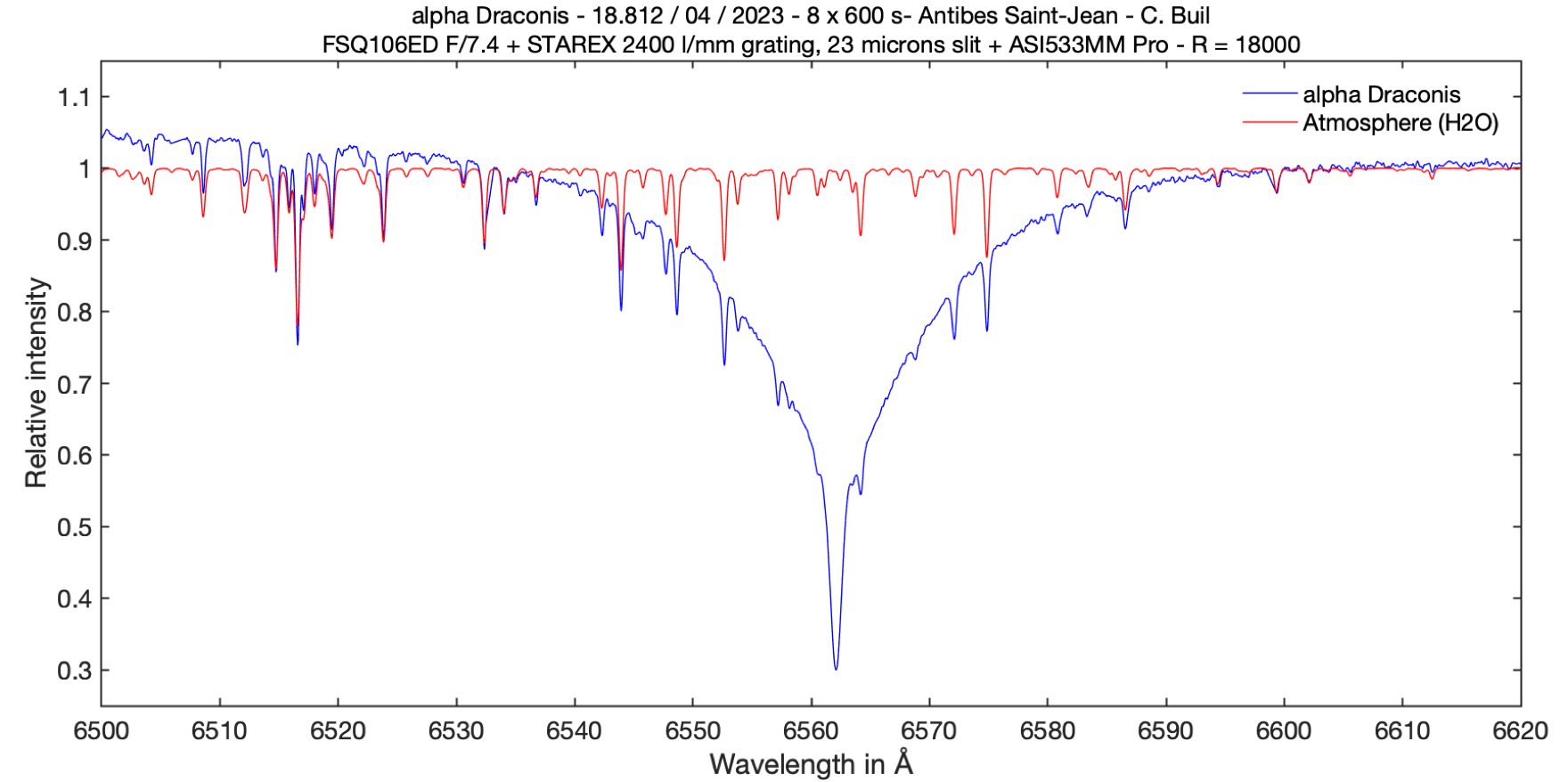
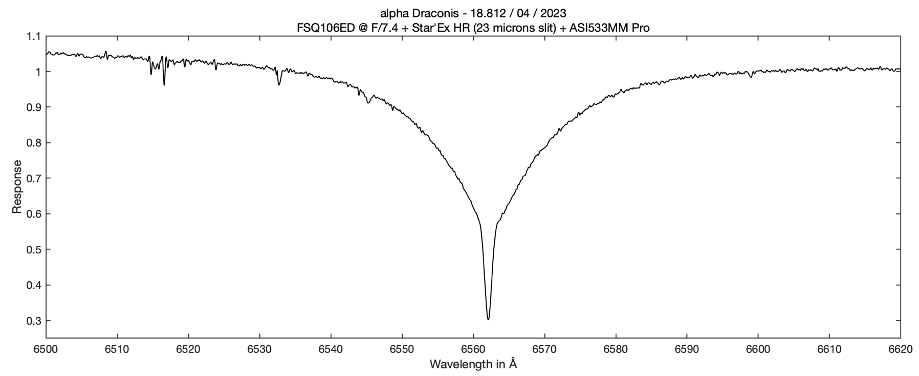
For your information, the function "_pro_telluric" saves the adjusted atmospheric file (red curve above) under the name "@atmo" in the working folder. It is instructive to note that at the heart of the Halpha line are water vapor lines that impact the shape of the stellar line, admittedly very discreetly, but in a very real way. By dividing the blue spectrum by the red spectrum, we obtain this, the spectrum that would be seen without atmosphere or from a very dry place on Earth:
A shift of 0.01 Å in the spectrum is enough to perceive a shift between the two spectra being compared. To help you gauge a possible spectral shift, the "_pro_telluric" function also returns information on this shift (O-C - Observed - Calculated) as well as the spectral resolution found in the spectrum (this measurement from the telluric lines is quite accurate as long as the said lines are present with good contrast).
The strange shape of the Halpha line, with two slopes, is called a Voigt profile and is very well explained by astrophysical phenomena.
To finish and complete the answer to the question, you have noticed that in the lateral calibration mode 4, a calibration polynomial must be provided as an argument to the "calib_coef" parameter. There are several ways to find these coefficient values, for example by using the lines of the neon lamp. But we will do better here by using again the telluric lines to evaluate their values.
The ideal is to use the spectrum of a bright and hot star (spectral type A or B) in which the Halpha line is blunted by the rapid rotation of the star on itself. The stars Regulus or Altair are very good candidates.
In a raw image of the spectrum of these stars, locate some relatively isolated and contrasted telluric lines. You can use the telluric lines map presented at the very beginning of this answer to identify them. For each of the selected lines, you will note the horizontal X coordinate to the nearest 2 or 3 pixels (no need to be very precise).
Tip: if you have difficulties to find the telluric lines in the 2D image of the spectrum, which is not abnormal, draw a raw profile in express mode of the image of this spectrum by using the special mode -5 (you should get used to using the special modes of specINTI, they can often help you, see the reference manual).
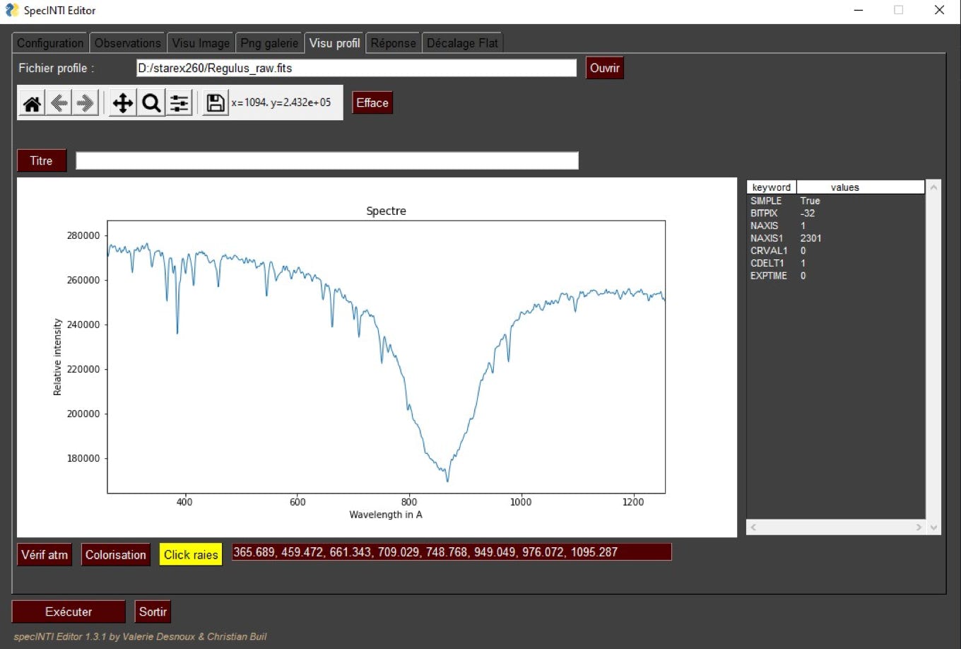
Another useful tip, this time related to the specINTI Editor interface. Let's suppose that you display the raw profile, but also any other profile (processed for example) from the "Profile view" tab. If you want to get a list of X-coordinates of a series of points in this displayed profile, nothing could be easier. Click on the " Click lines " button, which then turns yellow, and then click on the points you want in the profile with the left mouse button pressed down. The sequence of X coordinates of the selected points is displayed in a text box (you can copy it as needed after selecting it with the mouse and clicking "Ctrl C"):
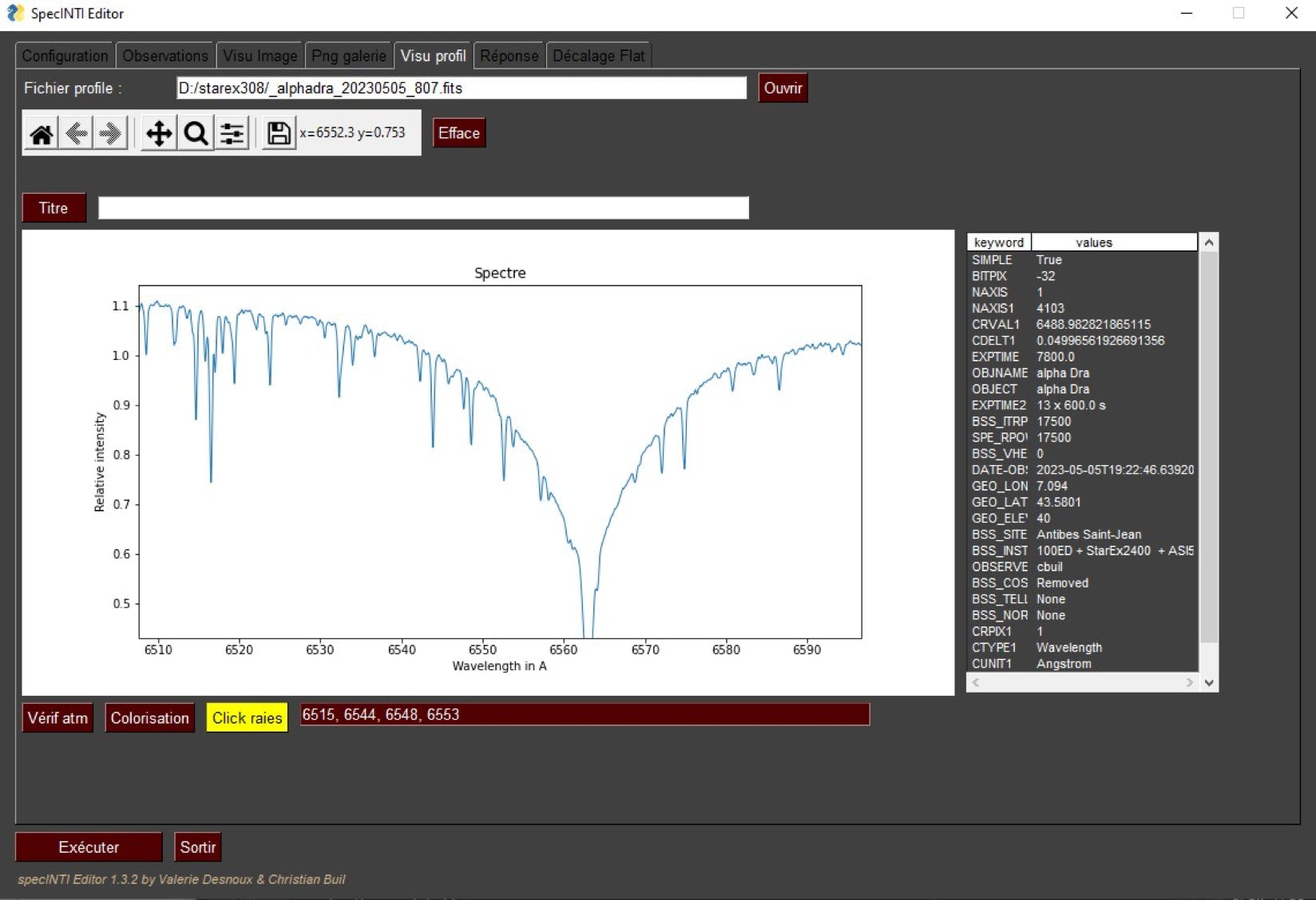
In our case, you can find the coordinates (in pixels) of the telluric lines that will be used to evaluate the calibration law.
Let's suppose that you have selected the following telluric lines, identified here by their wavelengths (see the relation with the graphical map of the spectrum of these lines given at the beginning of the answer) (note that we did not use the telluric lines located in the heart of the Halpha line, because this one, by its shape, can degrade the accuracy of the calculation):
[6514.738, 6523.850, 6543.912, 6548.627, 6552.632, 6572.087, 6574.860, 6586.559]
In comparison, we found the position of these lines at the following X coordinates (this is an example of course):
[367, 459, 661, 709, 748, 949, 976, 1095]
It is now easy to estimate a scattering law from this information. To do this, you create a mini configuration file that exploits the special mode -11 (see here again the reference manual):
# ---------------------------------------------------
# Special mode -11
# Exploitation of the -11 mode for the evaluation of the calibration polynomial from the telluric lines
# ---------------------------------------------------
# ---------------------------------------------------
# Working directory
# ---------------------------------------------------
working_path: D:/starex260
# ---------------------------------------------------
# Processing batch file
# ---------------------------------------------------
batch_name: regulus_mode-11
# ---------------------------------------------------
# Spectral calibration mode
# ---------------------------------------------------
calib_mode: -11
# ---------------------------------------------------
# Order of the polynomial to evaluate
# ---------------------------------------------------
poly_order: 2
# ---------------------------------------------------
# Wave lengths and X coordinates of telluric lines
# ---------------------------------------------------
wavelength2: [6514.738, 6523.850, 6543.912, 6548.627, 6552.632, 6572.087, 6574.860, 6586.559]
line_pos2: [367, 459, 661, 709, 748, 949, 976, 1095]
# --------------------------------------------
# Binning width
# --------------------------------------------
bin_size: 30
# ---------------------------------------------------
# Sky background calculation areas
# ---------------------------------------------------
sky: [200, 20, 20, 200]
# ---------------------------------------------------
# Sky extraction mode
# ---------------------------------------------------
sky_mode: 0
# ---------------------------------------------------
# x-terminals for geometric measurements
# ---------------------------------------------------
xlimit: [300, 1500]
# ----------------------------------------------------------------
# Width in pixels of the line search area
# spectral calibration
# ----------------------------------------------------------------
search_wide: 22
On the side of the corresponding observation file, you can be satisfied with the minimum (in the example, I do not even use the flat-field, for example) :
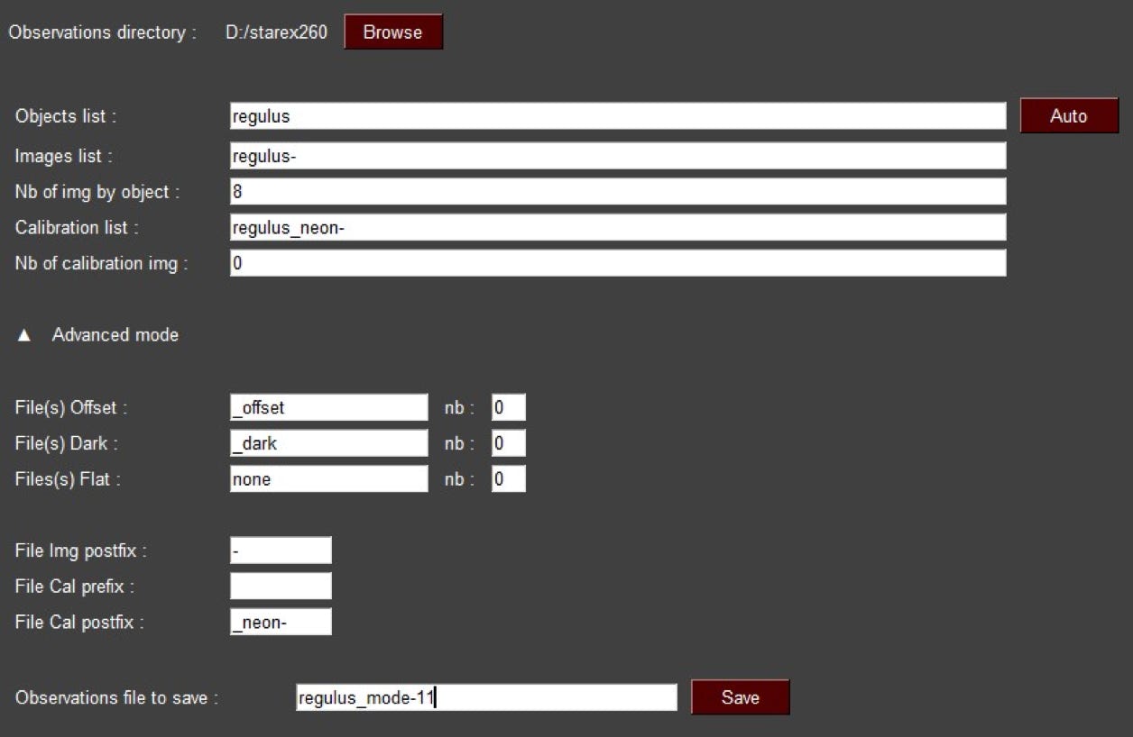
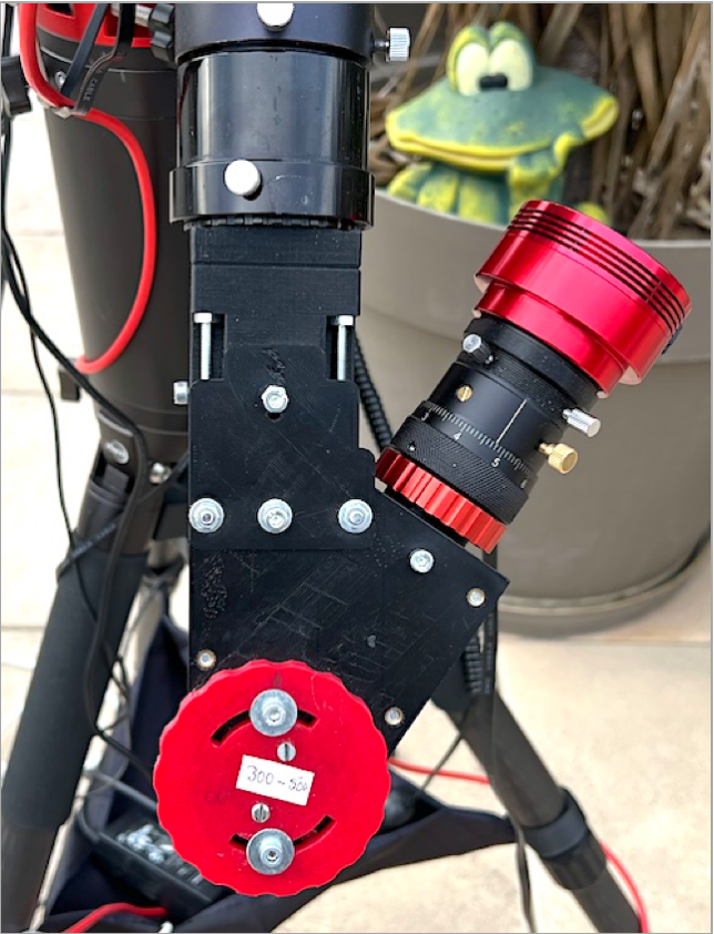
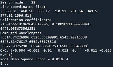
For example, here is what specINTI returns when run with this configuration file:
All that remains is to copy the values "-1.0166619e-06, 0.1001091, 6578.0587" as an argument to the "calib_coef" parameter in mode 4:
calib_coef: [-1.0166619e-06, 0.1001091, 6578.0587]
Two important remarks: (1) These coefficients are constants of the spectrograph and if you do not strongly deregulate it, you will not have to recalculate them. Therefore, this relatively cumbersome procedure will only be a formality in your normal use of the instrument. (2) Establishing the dispersion polynomial over a relatively wide spectral range from the telluric lines, rather than in a narrow range as when using the neon lines, provides a more wavelength-covering and accurate calibration. This point is important when the spectrograph is subject to a chromatic aberration a little strong, as with a Lhires III, but Star'Ex, better corrected, also benefits from this advantage
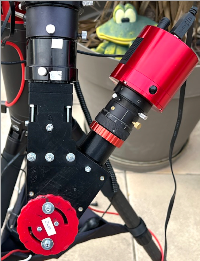
Since we are talking about high spectral accuracy in this answer, it is difficult to dissociate this accuracy from the signal to noise ratio in the spectrum. Automatically, the higher the signal-to-noise ratio (low noise to signal ratio), the better the spectral calibration. So, if you are looking for the ultimate accuracy when measuring a radial velocity, consider using long exposure times (within reason, because after an hour to an hour and a half of cumulative exposure, the SNR gain shows only a slow increase in general).
Since version 2.2.0 of specINTI, you have a little tool to find the SNR in the form of a parameter that you can add wherever you want in the configuration file (for example, in a "goodies" section). This is the "snr" parameter with as argument the spectral interval in angstroms within which the signal value, the noise value, and finally the signal to noise ratio is calculated. This interval must be chosen in a part of the continuum free of spectral lines, neither too wide nor too narrow. For example, add the following line to your configuration file:
snr: [6550, 6665]
In the output console, at the end of the processing, specINTI outputs the (approximate) SNR found in this part of the spectrum:
A4.4 : The Earth is animated by a proper speed while orbiting the Sun, how to take into account this fact to find a consistent radial velocity between observations of the same celestial object ?
The Earth orbits at a speed close to 30 km/s around the Sun. Depending on how the pointed object is oriented with respect to the plane of the Earth's orbit, its apparent radial velocity will be affected by this motion of the Earth. The amplitude and sign of this perturbation change according to the position of the object in the sky and the time of the year. A speed also depends on the positioning of the planets Jupiter, Saturn ... which modifies the orbit of the Earth. The calculation is therefore quite heavy.
But the situation is even more complex when we want a high precision. It is necessary to take into account the daily training of the observer on the surface of our planet: high speed at the equator and canceling at the poles ... To go even further, it is the speed generated by the Earth-Moon couple that must be considered. It is at this price that we can evaluate the topocentric speed of the observer to correct to better than one meter per second in radial velocity of the objects in the sky (a precision typically needed for work on exoplanets, see better).
specINTI includes a function to correct the topocentric velocity of the Earth in order to bring it back to the situation of an observer at rest with respect to the studied star (at the center of the Sun precisely).
To do this, we need the date of the observation (accurate to a few seconds when looking for accuracies below the meter, but we will not go that far), the equatorial coordinates and the geographic coordinates of the observer.
The date is searched in the DATE-OBS field of the FITS header of the first spectrum image of a sequence (a date in Universal Time).
The equatorial coordinates are taken from the header of the FITS file of the first image of a sequence, in the keywords CRVAL1 (right ascension) and CRVAL2 (declination). If these keywords are not present, the last chance is to query SIMBAD to find the coordinates by object name. This requires access to the Internet.
Finally, the geographical coordinates are the values of the parameters longitude, latitude, altitude, which are specified in the configuration file.
To indicate that you want to correct the wavelengths of the processed spectrum of the topocentric speed, you must define the parameter "corr_topo", with the proper radial speed of the object in km/s as value (if this radial speed is not known, indicate the value 0). By definition, if the object moves away from us the speed is positive, if it approaches us, the speed is negative. For example, the radial velocity of the star alpha Draconis is -13,0 km/s (see on SIMBAD) and we write :
corr_topo: -13.0
If the equatorial coordinates are not in the FITS header because the acquisition software has not entered them automatically (a frequent case unfortunately), you must then add the command "simbad" in the configuration file, with for example (the order does not matter) :
simbad: 1
corr_topo: -13.0
The software will search for the coordinates 2000.0 on SIMBAD. You will then find lines in the output console that look like this:
Radial velocity correction...
SIMBAD query for equatorial coordinates...
Alpha: 211.097 deg.
Delta: 64.3759 deg.
Topocentric velocity: 7.963 km / s
Object toward the Earth by : -5.037 km / s
This means that a correction of -5.037 km / s is applied to all wavelengths of the spectrum (here, the object is approaching us at a speed of 5 km / s per second, which produces a blue shift of the spectral lines).
Note 1: it can happen that the name of the object studied is not recognized by SIMBAD (outburst, supernova, comet...). specINTI then offers a way to get out of this bad situation by allowing to provide the name of an object (recognized by it) located not far from the target, via the parameter "near_star". Example :
simbad: 1
near_star: HD122363
corr_topo: -13.0
Note 2: most observing programs require that the heliocentric or topocentric velocity correction not be applied to the data. However, the "corr_topo" parameter is particularly important if you are trying to interpret a set of spectra of a time sequence by yourself. But, it is important, if you have to deliver your spectra to a database like BeSS or STAROS, for example, do not put this parameter in your configuration file.
Note 3: In addition to the tool integrated into specINTI, you can also evaluate barycentric speed from a web application: https://astroutils.astronomy.osu.edu/exofast/barycorr.html
A4.5: The apparent spectral signal depends on the optical transmission of the atmosphere, how to erase this phenomenon?
Indeed, depending on whether the same star is close to the horizon or located at the zenith, the shape of its spectrum is not the same. The earth's atmosphere absorbs the light as much as the object is located at a low elevation, and also more as we go towards the blue part of the spectrum. This effect of atmospheric transmission is often a source of difficulty when it comes to evaluating the true signal of the star, as it would be seen if the atmosphere were absent.
The spectral absorption of the star's radiation is a parasitic effect that is however quite easy to calculate and therefore to eliminate. The idea is to perform the following operation:
spectrum outside the atmosphere = apparent spectrum / atmospheric transmission
This operation is important in low resolution spectrography, and is a preliminary to the calculation of the instrumental response, as explained in section 7 of the specINTI documentation. The software performs the previous operation for you by giving the parameter "corrr_atmo" the value of the AOD. For example :
corr_atmo: 0.10
A complication comes from the fact that this function requires the geographical coordinates of the star in addition to the geographical coordinates of the place of observation and the date. As for "corr_topo" (see A3.4), if the equatorial coordinates are not in the header of the image files, you can query SIMBAD, by doing for example :
simbad: 1
corr_atmo: 0.10
Note: you can also provide the name of an object recognized by SIMBAS if the name of your target is not recognized by SIMBAD (outburst, supernova, comet...). Use then the "near_star" parameter. Example :
simbad: 1
near_star: HD122363
corr_atmo: 0.10
specINTI integrates a variant of the "corr_atmo" parameter, which has two arguments, in order the value of the AOD and the angular height of the object (evaluated elsewhere, and therefore the equatorial coordinates of the star are not necessary). This is the parameter "corr_atmo2). For example :
corr_atmo2: [0.10, 43]
A4.6 : How to calibrate a spectrum obtained without slit ?
Slitless spectrography is when the traditional narrow entrance slit of the spectrograph is removed, or replaced by a wide slit, several tenths to several millimeters wide. The goal is to make a spectrum in the simplest way possible, like a photograph, by positioning the target star approximately in the center of the field, with the help of a good finder in parallel with the main instrument; which can also have a self-guiding function. The absence of a fine slit guarantees that the maximum signal is available to produce the spectrum. The spectrophotometric quality of the data is also very good (no more problems of atmospheric or instrumental chromatism that induces artificial distortions in the continuum of stars).
A gauche, Star’Ex configuré en mode « spectrographie sans fente » basse résolution. A droite, on travaille en haute résolution (configuration proche de Sol’Ex). Noter l’absence d’un système de guidage à l’entrée du spectrographe.
In addition to the rise of the sky background because of the absence of the slit, the other major drawback of this solution is the difficulty to calibrate the spectra in wavelength because nothing guarantees that from one object to another we will be at the same position at the entrance of the spectrograph. It is also impossible to use an emission line lamp, the spectrography without slit being possible only with point objects (stars).
In low resolution spectrography we can use the Balmer lines of a hot star to find the dispersion law, then this recalibrate on a detail of the spectrum of other objects through a simple translation in wavelength. The difficulties are greater in high resolution spectrography. The reasonable solution is to use the telluric lines, for example those present around the Halpha line (by chance in this case).
We proceed in four steps (be careful, we exploit here advanced functions of specINTI, which can give you other ideas if used):
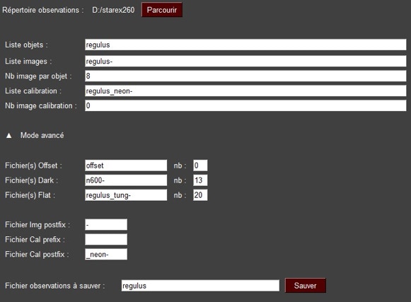
Step 1: extraction of a raw (uncalibrated) profile from the spectral images, themselves raw. This is done using the -5 spectral calibration mode. In this mode, specINTI simply performs the classic pre-processing (offset, dark), if you wish, performs geometric corrections at your request and finally performs a binning operation. The result is a profile file xxxx_raw.fits, not calibrated in wavelength and with intensity in ADU units (all the spectrum signal integrated for each column). Here is the observation file for a sequence of 8 images of the star Regulus realized without slit in high resolution with a telescope of 80 mm (exposures of 60 seconds):
The configuration file is simple:
# ---------------------------------------------------
# Répertoire de travail
# ---------------------------------------------------
working_path: D:/starex260
# ---------------------------------------------------
# Fichier batch de traitement
# ---------------------------------------------------
batch_name: Regulus
# ---------------------------------------------------
# Mode d'étalonnage spectral
# ---------------------------------------------------
calib_mode: -5
# --------------------------------------------
# Largeur de binning
# --------------------------------------------
bin_size: 30
# --------------------------------------------
# Retrait du fond de ciel
# --------------------------------------------
sky_remove: 1
# ---------------------------------------------------
# Zones de calcul du fond de ciel
# ---------------------------------------------------
sky: [200, 22, 22, 200]
# ---------------------------------------------------
# Mode extraction du ciel
# ---------------------------------------------------
sky_mode: 0
# ---------------------------------------------------
# Bornes x pour mesures géométriques
# ---------------------------------------------------
xlimit: [400, 1700]
# ----------------------------------------------------------------
# Motif de filtrage médian
# ----------------------------------------------------------------
kernel_size: -3
# ----------------------------------------------------------------
# Filtrage gaussien
# ----------------------------------------------------------------
sigma_gauss: 1.0
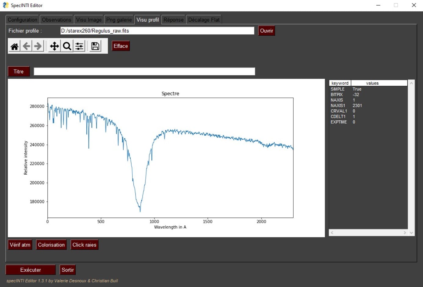
We notice the value of the "calib_mode" parameter, which is -5 here. Some noise filtering is done, but it is optional (kernel_soze, sigma_gauss). Here, the result is the file "Regulus_raw.fits":
Tip: the -5 mode can be used at the same time as the observation or for some analysis in order to quickly evaluate the signal present in the spectrum in ADU and possibly bring a retouch (focusing for example).
Step 2: Locate some telluric lines and record their positions in pixels. Here is a map of telluric lines (H2O) usable around the Halpha line:
From version 1.3 of specINTI Editor you have a tool (button "Click lines") that makes a list of points that you click in the profile, here at the level of telluric lines (no need for a paper to note, think also that you can zoom in the profile):
Step 3: we calculate from this list of points the dispersion polynomial passing best among them. We use the calibration mode -11, which is close to the mode -1 (calibration from a set of absorption lines), but simpler because it is not necessary to have a calibration lamp (extract):
# ---------------------------------------------------
# Répertoire de travail
# ---------------------------------------------------
working_path: D:/starex260
# ---------------------------------------------------
# Fichier batch de traitement
# ---------------------------------------------------
batch_name: regulus
# ---------------------------------------------------
# Mode d'étalonnage spectral
# ---------------------------------------------------
calib_mode: -11
# ---------------------------------------------------
# Ordre du polynôme a évaluer
# ---------------------------------------------------
poly_order: 2
# ---------------------------------------------------
# Liste des raies à ajuster
# ---------------------------------------------------
line_pos2: [365.689, 459.472, 661.343, 709.029, 748.768, 949.049, 976.072, 1095.287]
wavelength2: [6514.738, 6523.850, 6543.912, 6548.627, 6552.632, 6572.087, 6574.860, 6586.559]
# ---------------------------------------------------
# Angle de slant
# ---------------------------------------------------
slant: 0
# --------------------------------------------
# Largeur de binning
# --------------------------------------------
bin_size: 33
# ---------------------------------------------------
# Zones de calcul du fond de ciel
# ---------------------------------------------------
sky: [200, 20, 20, 200]
---------------------------------------------------
# Bornes x pour mesures géométriques
# ---------------------------------------------------
xlimit: [300, 1500]
# ----------------------------------------------------------------
# Largeur en pixels de la zone de recherche des raies
# d'étalonnage spectral
# ----------------------------------------------------------------
search_wide: 22
The important part is the "line_pos2" parameter, which takes the coordinates previously found interactively in the profile (copy and paste). The "wavelength2" parameter is a list of the corresponding wavelengths (see the telluric lines map).
After launching the program, we find here (output in the console) :
It appears that in the area of the spectrum considered, the calibration error is very reliable (calibrating from information present in the spectrum that we process is ideal because we minimize the bias, or pseudo noise).
Step 4: it only remains to process our spectrum in the rules of art using the mode of calibration 1 (based on a calibration polynomial). You just have to write the following line, which uses the coefficients previously calculated:
calib_coef: [-1.0166619196264581e-06, 0.1001091180029949, 6478.058673562251]
A4.8 : I have a very bright telescope, open at f/4, can I use it with Star'Ex and what are the specificities of the treatment ?
The answer to this question cannot be unique. In particular, it is important to distinguish between the category of spectrography practiced: low spectral resolution or high spectral resolution. The requirements are not the same while the coupling between the spectrograph used and the telescope with which it is associated also has a very direct impact. It is usual to say that there is no universal spectrograph for all subjects and all telescopes. All this makes it difficult to answer.
A spectrograph such as Star'Ex offers a lot of flexibility and adaptability, but it too has limitations in this exercise. In fact, we have to take the problem in reverse: I have a given spectrograph and I want to use it in a given way (low or high spectral resolution to make it simple), which telescope should I use to get the most out of it.
Another difficulty is that in spectrography the results are often counter-intuitive, with answers that can confuse. This is what the question asked leads to. The experiment allows to answer it, but it is also good to be confronted with the reality of the figures, which is less subjective and shows more clearly the weakness or quality of the technical configurations retained.
The best way to compare the configurations between them is to calculate the equivalent surface of its telescope by taking into account a number of parameters. The surface of the mirror is indeed little representative of the final result.
Let's take the example of a Newton Sky-Watcher Quattro telescope of 150 mm diameter (D) and open at f/4, a popular and economical model.
We want to work in high spectral resolution with Star'Ex to reach a resolving power of about R=19000 at the Halpha line due to hydrogen. To do this, we must use a relatively narrow slit. We fix on the "standard" value of 19 microns (a width proposed by the multiple slit Shelyak), and which in fact, allows to reach a resolving power of R = 23000 with Star'Ex, but we assume that the treatment applied brings us back to R = 19000 (light filtering of noise by Gaussian convolution). We assume that the seeing is poor, that we are not very comfortable with the focusing of stars on the slit and with the autoguiding. We fix on a seeing of 6 arc seconds, which means that in long exposure, the apparent width at half height of the stars is 6 arc seconds.
Let's first calculate the collecting surface of the telescope, with a diameter of D = 15 cm. The problem with the chosen model is that it is designed for wide field photography, which means that the secondary mirror is very large. We find here a central obstruction of the primary mirror of e = 0.43, which is quite enormous (note that you will not find this information in the manufacturer's documentation, it is not specified!) The effective collecting surface at the entrance of the telescope is thus :
S = 3.1416 x D^2 / 4 x (1 - e^2) = 144 cm2
Let's return to our seeing of 6 arc seconds. These are poor conditions for observation, but more frequent than we think. The focal length of the telescope being F = F# x D = 4 x 150 = 600 mm, the linear size of stars at the entrance of Star'Ex is :
FWHM = 600 x tan(6 / 3600) = 0.017 mm = 17 microns.
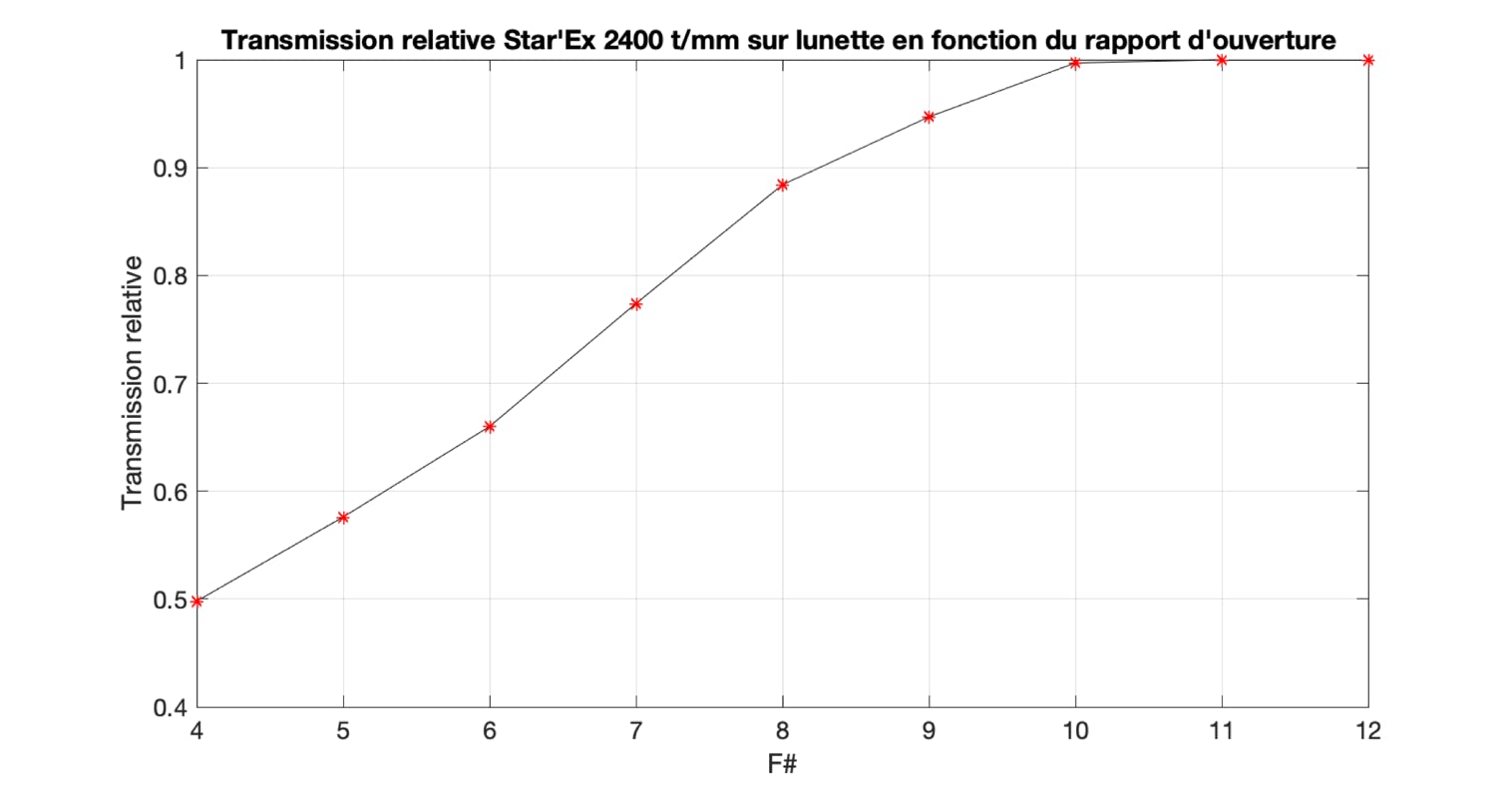
Here is a curve that shows the transmission of a slit of width w, while the images of the stars have a width FWHM (and a form of Gaussian function) :
How to read this curve? Let's assume that the FWHM of the stars and the slit width (w) are identical, then we have w/FWHM = 1, and the curve tells us that the spectrograph lets pass 0.76 times of the incident flux. This is a typical value in spectrography, rather good. In our case, with a FWHM of 17 microns, the result is even better with w/FWHM = 1.12, because we then find a slit transmission of Tslit = 0.81.
But the story is not so idyllic unfortunately.... We must now analyze the characteristics of the spectrograph, here Star'Ex. With the grating of 2400 lines/mm, the rays arrive on it with a high incidence because this optical surface is strongly inclined. Also, in the incident plane, the optical vignetting rises quickly when the telescope opens (increasingly bright). Very aggravating in our situation: the strong central obstruction of the telescope produces a shadow in the middle of the grating, where on the contrary we would like to have a maximum of light. Here is a curve calculated with the Zemax optical software in the situation of Star'Ex HR and a central obstruction of 0.43 which shows the rate of optical vignetting as a function of the F/D ratio (F#):
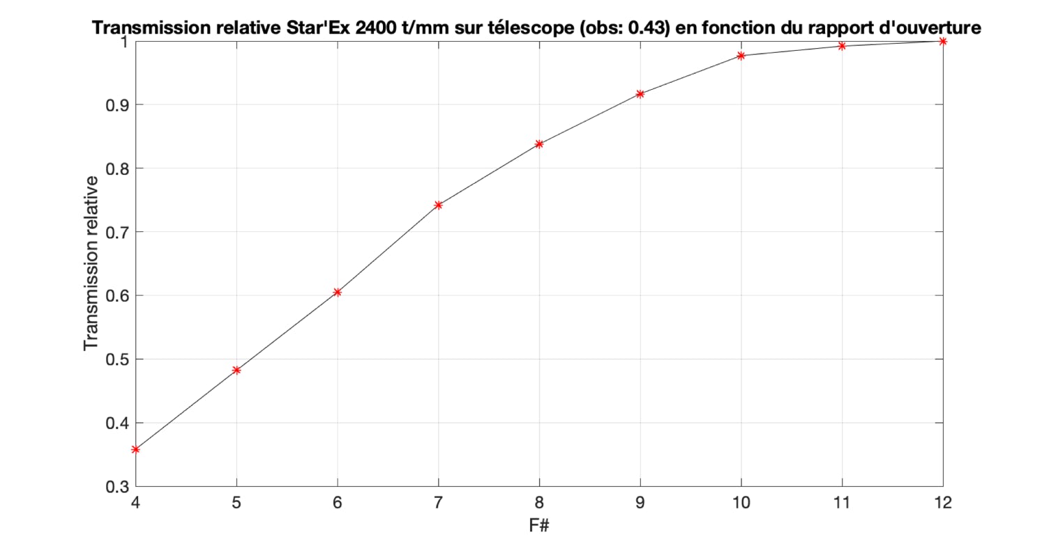
If the telescope was opened at F/10, the optical vignetting would be quite negligible. But we are at f/4, which induces a very severe vignetting of Tspectro = 0.36.
Another factor intervenes, the reflection coefficient of the mirrors. This is a parameter that is often forgotten when buying a telescope! Here, it is a question of an economic model, with a simple layer of aluminum protected. Taking into account the fact that we have two mirrors, the incidence on the secondary and a slight effect of polarization, we estimate that the optical transmission of this set of two mirrors is Topt = 0.80 (the author has made measurements, he even finds a slightly lower result, but we adopt here the theoretical value). This means that the mirrors of a basic telescope typically lose 20% of the incident flux simply because of the reflection coefficient. This is hard, but it is the reality.
In the end, the true effective surface of our telescope is :
Seff = S x Tfente x Tspectro x Topt = 144 x 0.81 x 0.36 x 0.80 = 34 cm2
This means that you have purchased a telescope of 150 mm in diameter but it has the output of a small telescope of 66 mm in diameter in the chosen configuration! This is quite dramatic.
To improve the situation a first lever is to reduce the effect of internal vignetting of the spectrograph. To do this we add a Barlow lens to the front of Star'Ex. We choose an economical x2 model from Kepler, which we use in an expeditious way in this way:
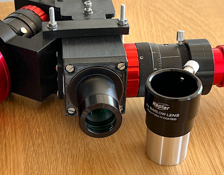
Given the distance between the lens and the slit in this case, the Barlow works at x2.3. The focal length is therefore increased to F = 2.3 x 600 = 1380 mm, and the F/D ratio increases to 9.2.
In these conditions we have Tfente = 0.42 (because w/FHM = 0.475), Tspectro = 0.83 (see curve), Topt = 0.80, hence a new effective surface of,
Seff = 144 x 0.42 x 0.92 x 0.80 = 44 cm2
This is better, but we notice that what we gain in terms of reduction of optical vignetting is lost for a good part by the enlargement of the image of the stars at the focus compared to a slit that does not change, and a loss of significant slit transmission. We are stuck!
Here is a first conclusion: in instrumental spectrography, whether it is Star'Ex or the huge spectrographs installed at the focus of the VLT telescope in Chile (ESO), for a given spectral resolution, the more the size of the telescope increases, the more the size of the spectrograph must be increased. There is an almost linear relationship (and the volume increases with the cube of the size!). This explains the size of spectrographs at the focus of 8 meter telescopes, which are no better in terms of spectral resolution than a Star'Ex at the focus of an amateur telescope.
But our problem is a bit different here: we have the telescope and the spectrograph, and we need to choose the resolution power that allows a reasonably high efficiency. In this case, we will moderate our ambition by going from a resolution of R = 19000 to a resolution of R = 13000 (which remains high spectral resolution). We thus widen our entrance slit to 35 microns. As a result, with a seeing of 6 arc seconds we have w/FWHM = 35 / 40 = 0.875 and the slit transmission increases to Tslit = 0.70. In the end, the effective area in a configuration considered reasonable to achieve R=13000 with a 150 mm telescope at the base open at f/4 is :
Seff = 144 x 0.70 x 0.92 x 0.80 = 74 cm2
Or the equivalent of an aperture of 97 mm. This is the cruel reality of physics, but this is not shocking in spectrography (a spectrograph whose yield reaches 20% is already considered very efficient, and when the red shift of galaxies was discovered at Mount Wilson, the yield of the spectrograph used was 1%, or even less (the photographic plates were not very sensitive ...).
So, yes, a telescope opened at f/4 is usable, but you have to take precautions, and in particular aim at a reasonable resolution power and use a Barlow lens, which is never very comfortable, we must admit.
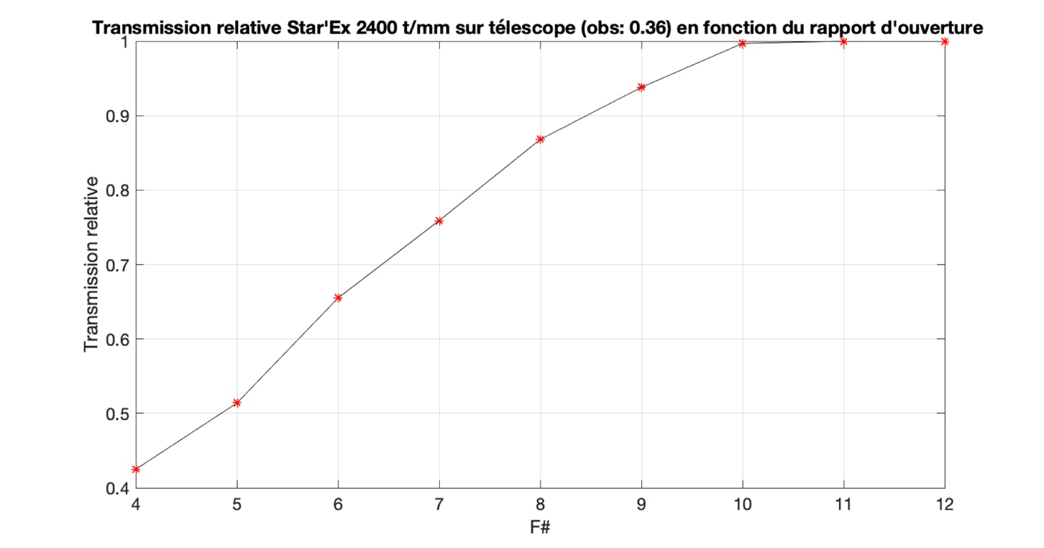
For information, here is the vignetting curve of Star'Ex HR with a Newton telescope whose central obstruction is only e = 0.36, which is still more reasonable than that of the famous Quattro SkyWatcher telescopes (this allows you to redo the calculations for your "setup" if necessary):
Can we do better with some refractors or telescopes in terms of ratio between the starting collecting area and the final effective area? The answer is yes, and this has a big impact on your purchases if you want to push towards efficient, easy to use and not too expensive spectrography 2.0. In the spirit of spectrography 2.0 it is a very good choice, for example the configuration favors nomadism, going on vacation with your equipment, etc. But this does not exclude of course the use of telescopes, we will see.
Spectacles have several advantages compared to telescopes as soon as we stay at a diameter of 100 mm, and not much more, that is to say in the spirit of a relatively economic spectrography (the V2.0):
- the refractors are more closed than the telescopes, which often avoids the inconvenient use of a Barlow
- the refractors are a little less sensitive to turbulence
- the optical quality is good, in particular in high resolution, where chromatism intervenes little because one works on a small domain of wavelength
- the refractors have an optical transmission of almost 100% (Topt = 1)
- the refractors have no central obstruction, which reduces the internal vignetting of the spectrograph, as shown by the following Star'Ex HR vignetting curve, precisely adapted for glasses (no central obstruction):
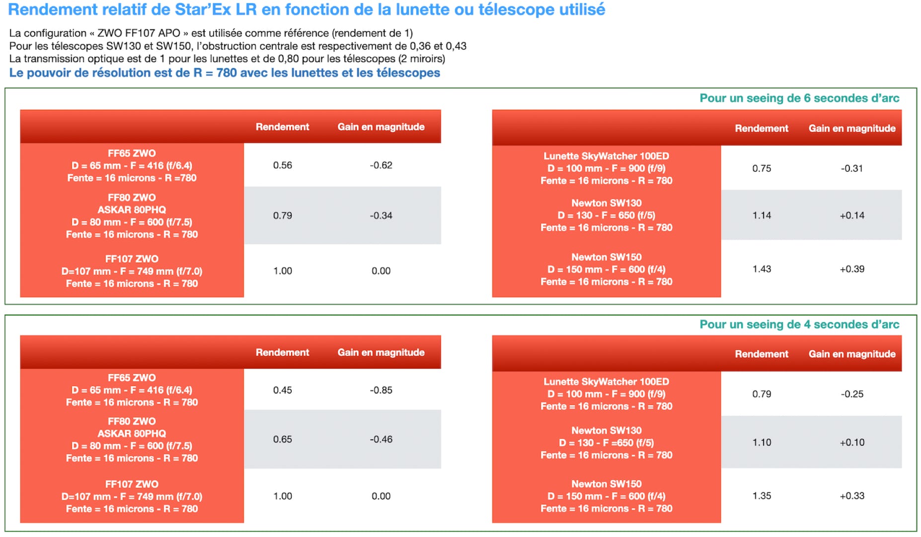
From all these elements it is quite easy to write a small computer code that evaluates your current equipment or your future purchases in spectrography (low-cost). The following table is a synthesis for some common configurations where I compare refracctor and telescopes. Note that for the scopes I have used the brand new FFxxx refractor from ZWO, which will surely become popular because of their price (but there are other criteria to choose from!).
I considered two situations for the seeing: a mediocre seeing of 6 arc seconds, a correct seeing of 4 arc seconds.
Finally, to facilitate the readability, I give the relative efficiency (or effective area) compared to a configuration based on the ZWO FF107 refractor. I also give the gain in consecutive magnitude.
Initially, to be as objective as possible, I considered that the power of resolution aimed is R = 19000, whatever the couple spectrograph / telescope or refractor:
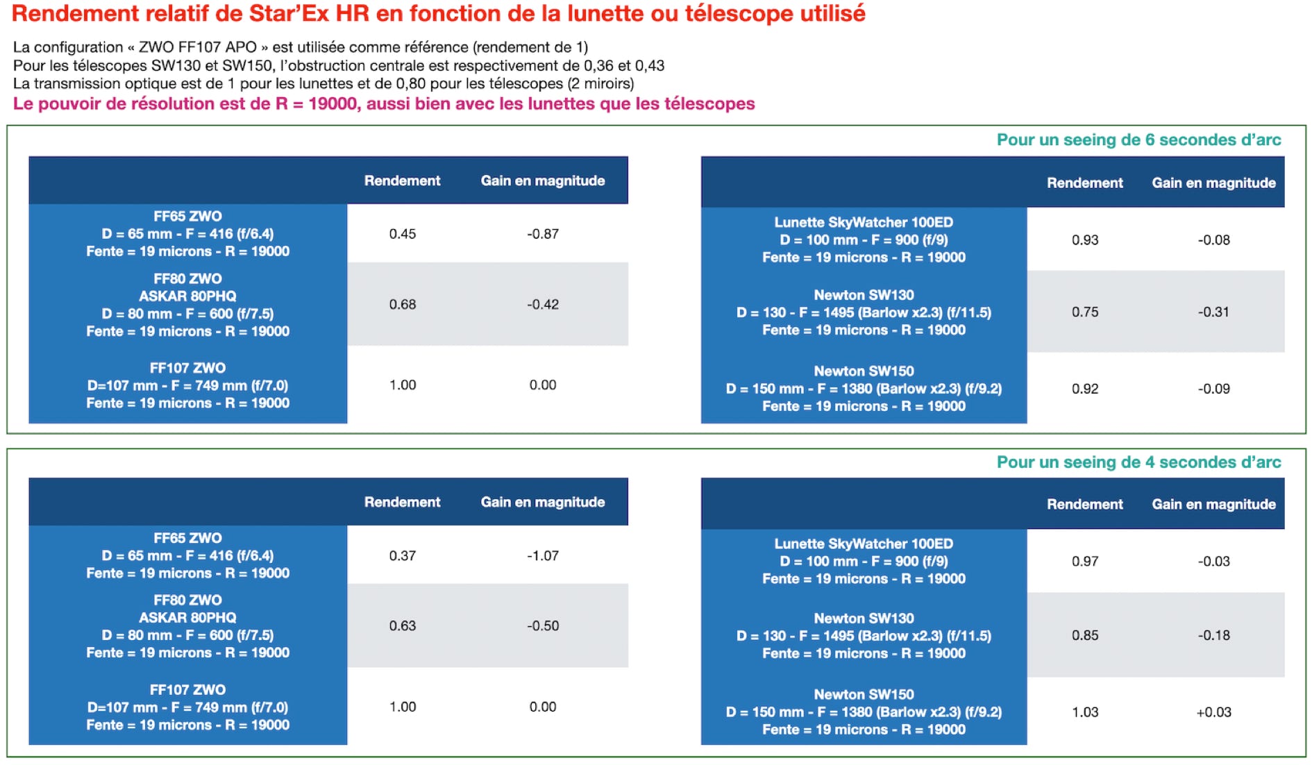
What does this table teach us in a few words (there is much to say). First, for the cases treated, the optimal configuration with Star'Ex HR is a 100 mm scope opened between f/7 and f/8. In raw performance, this is the best result. But there is an interesting subtlety to analyze. The ratio of the calculated efficiency between an 80 mm and a 107 mm refractor is here 0.68 (seeing of 6 arc seconds). But if we analyze the ratio of the physical surface of these instruments we find 80^2/107^2 = 0.56 only. This means that the 80 mm refractor, for its size and lower cost, offers a pretty good performance - this is the reason why the author often favors small instruments in spectrography, which are easier to use, more manageable, less demanding in terms of resources of any kind (as far as possible, because if one has to look for a supernova of magnitude 18, there is no other choice than to increase the diameter of the tube and especially to reduce the resolution power).
Another lesson, quite heavy, is that a 130 mm or 150 mm telescope does less well than a 100 mm telescope. This is a typical example of a counter-intuitive result. The equivalent area of a 100 mm telescope (or yield) is identical to that of a 150 mm telescope.
You have understood by reading the above, the resolving power must be adapted to the size of the telescope. We now consider a power of resolution of R = 19000 (so high) for the glasses and R = 12000 to 13000 for the telescopes considered (a lower resolution therefore, but very satisfactory for most studies, rest assured). Here is the result:
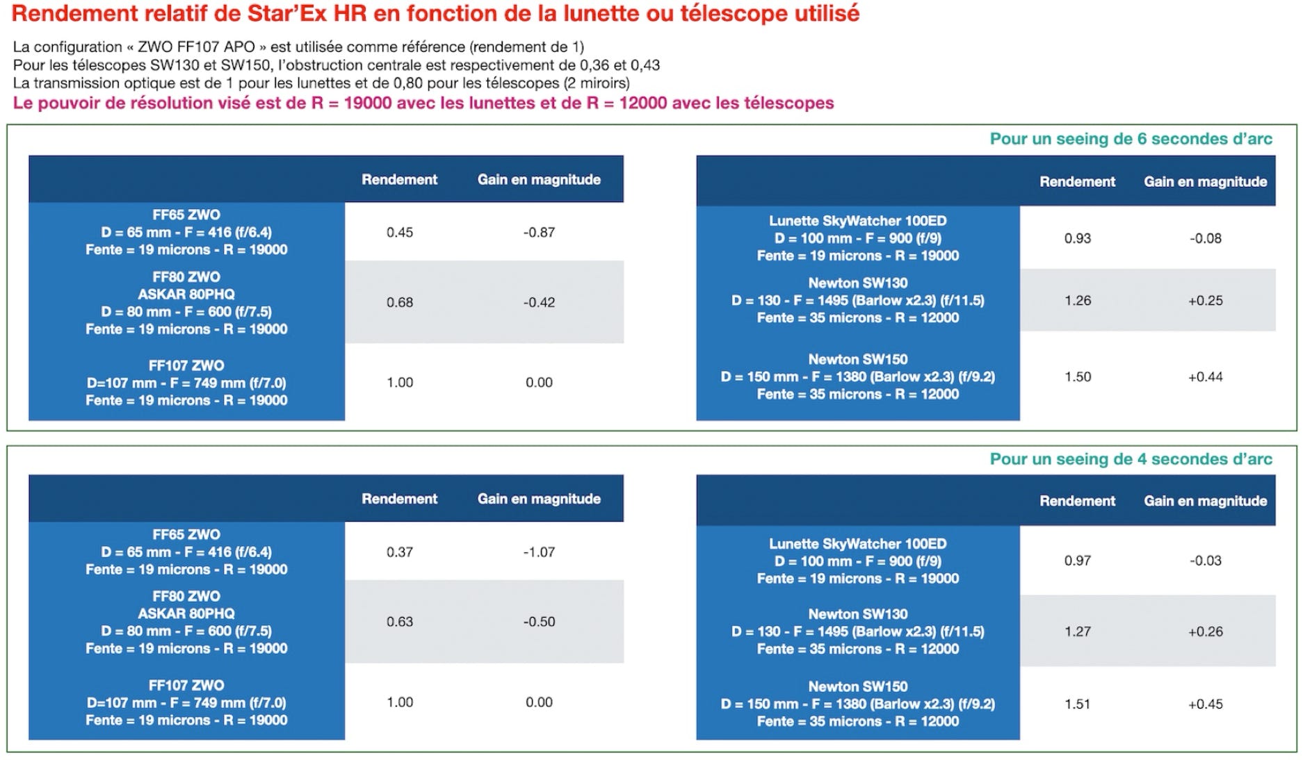
This time, the 130 mm and 150 mm telescopes take the lead. We see here the importance of the power of resolution that we give ourselves as an objective. Compared to an 80 mm refractor, the gain is about 1 magnitude, while compared to a 100 mm telescope, the gain is 0.5 magnitude (but once again, with a resolution power a little degraded, without being prohibitive). Admittedly, high spectral resolution with such an open telescope is a bit unnatural, even if nothing is impossible as seen here.

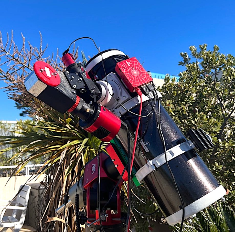
A gauche, l’aspect d’une lunette FSQ106ED exploite à la focale de 790 mm (utilisation d’une Barlow x1,49) sur une monture ZWO AM5. A droite, l’aspect d’un télescope de 150 mm Quattro exploité à la focale de 1380 mm (utilisation d’une Barlow x2,3), toujours sur une monture AM5.
And the low resolution you may say. It is quite possible to make the same calculations with a Star'Ex LR, aiming this time at a resolution power of about R=780 (16 microns slit). The calculation is simpler because the internal vignetting in Star'Ex is zero until f/5 and barely perceptible at f/4 (we adopt a Tspectro vignetting of 0.95 at f/4, a bit pessimistic). Following the same principle of calculation, here is the result for the same scopes and telescopes as in HR :
The gain offered by the 150 mm f/4 telescope is now significant (without having to add a Barlow of course, we work directly at the focus of the telescope, Star'Ex accepts it very well). We perceive here the difference of regime between high and low resolution. Note also that for the spectrography of objects with an extended surface (nebula, comets), a telescope opened at f/4 or f/5 will also offer a much brighter image than a telescope opened at f/7. This is a big plus, especially if the telescope is large in diameter (200 mm, 250 mm ...).
The Cassegrain or Ritchey-Chrétien telescopes are in an intermediate situation: no chromatism, which is perfect, but strong increase of the focal length when the diameter becomes high. We then have the obligation to reduce the power of resolution because of the enlargement of the slit. It's up to you to do the calculations (they are simple) for your current configuration.
Let us add that the chromatic aberration of the astronomical refractor, known as "APOchromatic", which often have only the name, is always more or less present. Some modern lenses with 3 or 5 lenses and special glasses produce a spectrum still relatively clear up to 3800 A, or even 3750 A. But in this field, perfection is obtained with a mirror telescope (without corrector) which by definition is achromatic, which is an asset in spectrography. The following document shows the aspect of the visible spectrum realized with a Star'eEx LR, top with a telescope that behaves well with respect to chromatism, and bottom, the spectrum of the same star (Vega) obtained with a Newton telescope 150 mm f/4 :

With a refractor, you have to deal with the widening of the track in the deep blue and ultraviolet part, but here quite contained (the TS refractor does a good job, it is a good product; you can find much worse). If the width of the binning area (parameter "bin_size") is chosen wide enough, it will include all parts of the spectrum, from blue to red. This is what must be done with care, when needed (no need to exaggerate the width either). Thanks to the optimized binning if the object is of low intensity ("extract_mode" parameter at 1) and despite this enlargement, the noise does not rise in the calculated spectral profile. What matters most here is that the spectral lines remain relatively fine in the near UV, despite the enlargement (presence of a stigmatism which is favorable to us). The optics of Star'Ex LR is calculated so that it is so (some Star'Ex users are mistaken when they buy the lenses in the catalogs of the suppliers of traditional optical components, because the result will be less good).
But the absolute weapon against chromatism is the mirror telescope. Despite this, in the spectrum shown, at the bottom of the figure, we still notice a broadening in the blue. Here it is Star'Ex itself that shows these limits (it is also made of lenses). But beware, in the example, the telescope is very open (the maximum for Star'Ex). This chromatic defect becomes discrete at f/5 and very discrete at f/6 and above. In this case (input beam at f/4), the spectrum is usable up to about 3800 A. Anyway, below 3700 A, some glasses used in the Star'Ex optical combination become almost opaque. Still in the example of the spectrum made with the telescope of 150 mm f/4, we notice a dark area in the middle of the trace and in the UV: it is the shadow of the secondary mirror that appears, the better the spectrum widens.
In summary, in any case with Star'Ex :
- For high spectral resolution, up to stars of magnitude 9 or so, prefer a small refractor of 80 to 130 mm in diameter open between f/7-f/9.
- For low resolution (novae, variable stars, supernovae, comets, nebulae...) prefer a Newton type telescope (or other) open between f/4-f/6. Avoid using an optical complement like Barlow or coma corrector is also ideal to avoid any chromatism of the telescope and other concerns of more or less fragile mounts (direct to the focus therefore, it is the recommendation).
A4.9: Is it possible to use an LED screen to make a flat-field in spectrography?
The answer is no in low spectral resolution, the spectral content of these lights is far from being spectrally uniform. It is far from the monotonic curve of a black body (incandescent lamp). This situation is unmanageable.
The answer is yes in high resolution under conditions. Here again the rather chaotic spectral distribution can be felt, but less urgently, because the spectral range is restricted.
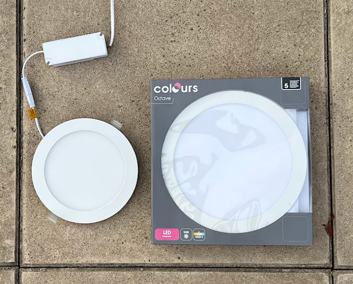
I recommend a LED source of this type, with a flat and homogeneous surface (all sizes are available in all DIY stores):
I use this type of source very commonly today, but only for high resolution (for example Star'Ex HR) and for the Halpha region. Here's what it looks like at night with a FQ106ED or a 150mm Newton (it's easy to cover with a small black sheet to avoid illuminating the environment, and I arrange a small counterweight above the panel so it doesn't slip, with the vertical telescope securely in place - you can do less rustic softbox things!):
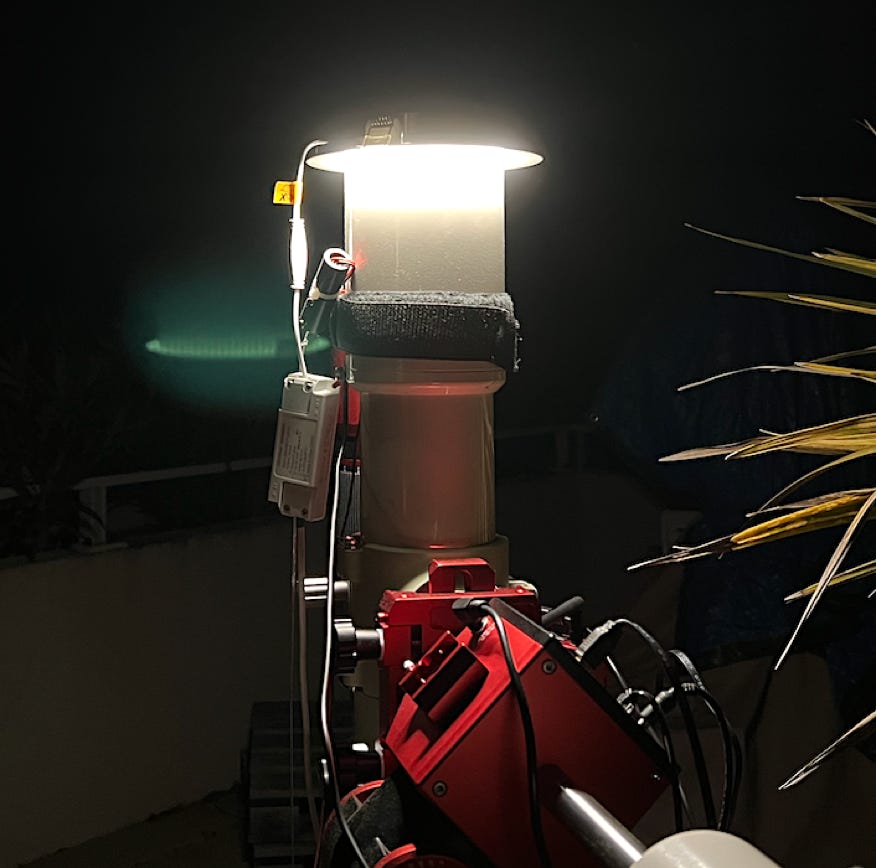
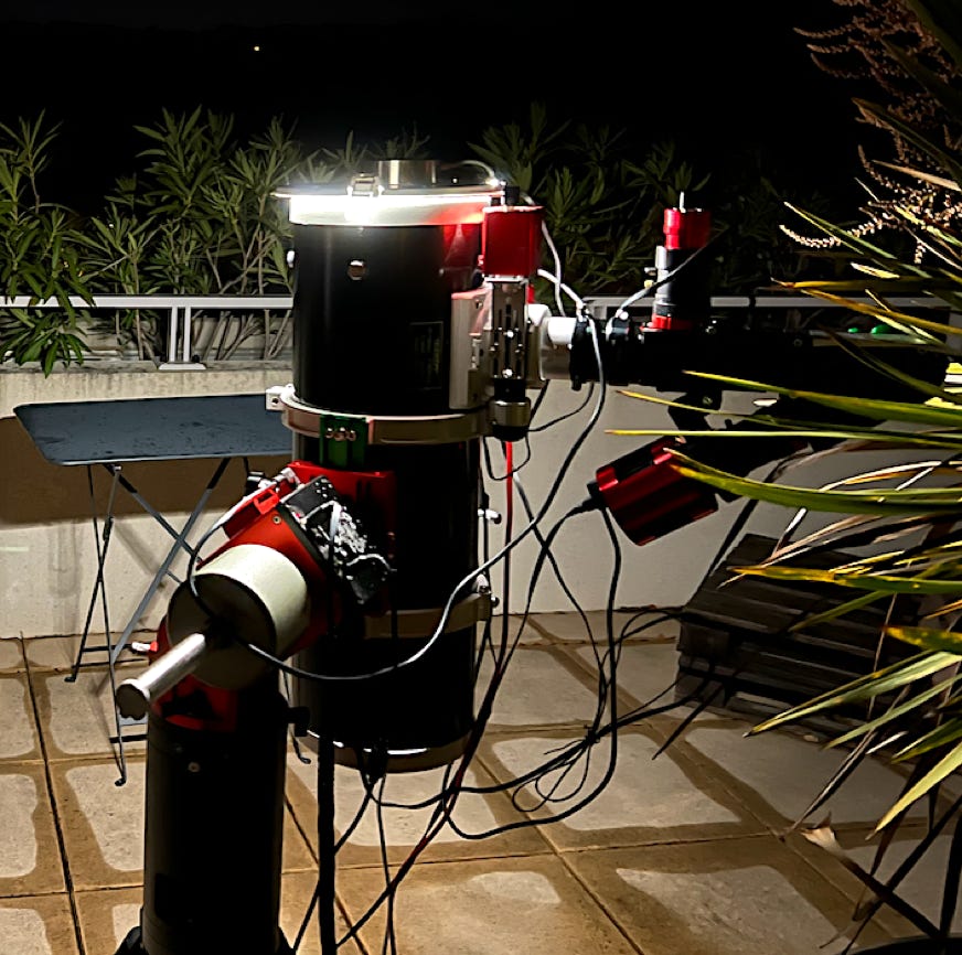
Contrary to the impression of a high intensity, the flux sent to 656 nanometers (Halpha line) is really weak. The spectral distribution is far from being white, this is the big concern of LEDs. With a Star'Ex HR, it takes typically 10 seconds of exposure to get the right signal in the flat-field. And even for a small spectral range there is a significant variation in the spectral distribution (almost a factor of 2 less on the red side compared to the blue side), but hey, these panels are easy and practical and the flat-field is correct, which is the main thing:
Given the spectral distribution, it's impossible to use the "Planck" parameter to get an approximately flat response. The response curve with LEDs is even inverted compared to a blackbody at 2700 K. Here is the typical response I get around Halpha with Star'Ex HR, an ASI533MM camera and given the type of LED illumination used (this is the spectral file provided as a parameter to "instrumental_response" in the configuration file):
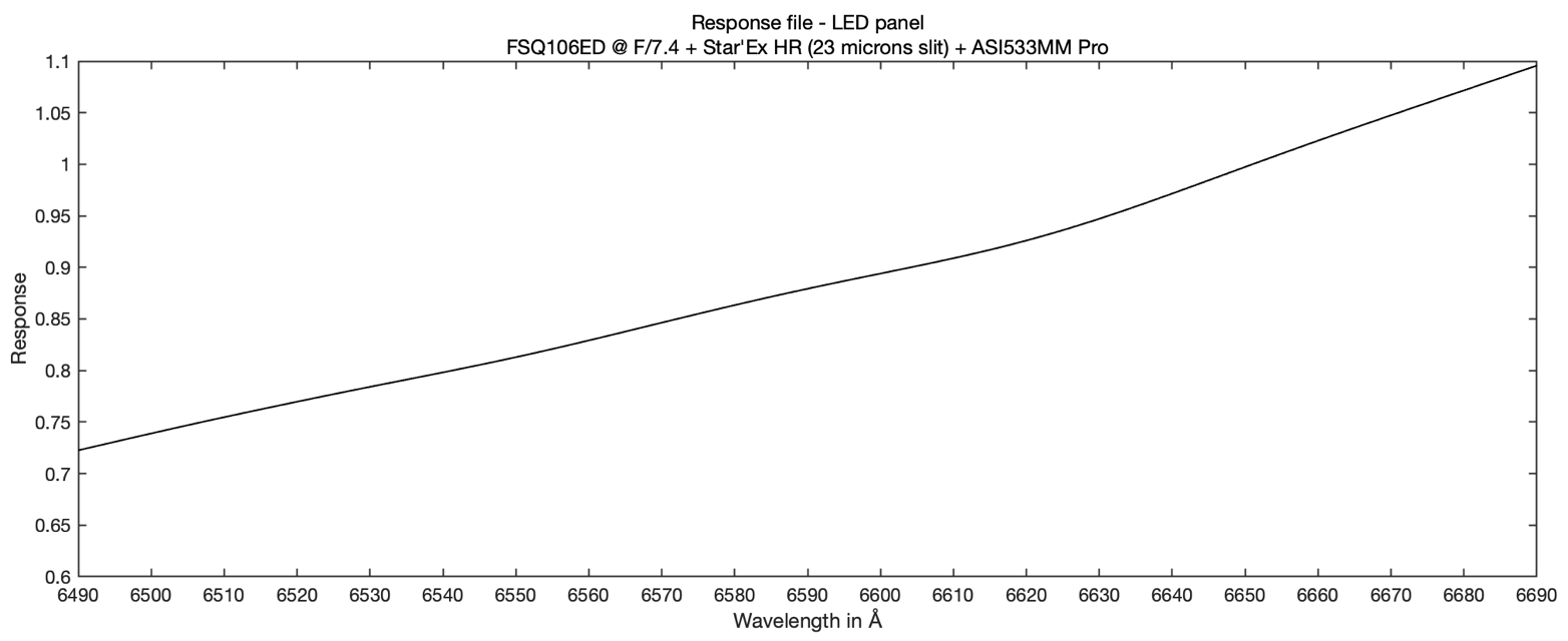
A4.10: What is the limiting magnitude I can expect when observing with a 100 mm telescope?
The answer depends on many factors. Of course, the spectral resolution adopted is critical. As the resolving power of the spectrograph increases, the more the light is diluted in the plane of the detector that records the spectrum and the more the noise ends up dominating the signal. A ratio between the signal and the noise (random fluctuation) equal to the value 3 in the spectral profile is considered as a limit threshold of effective detection of the signal. This threshold can be used to define the limit magnitude. A signal to noise ratio (SNR) of 5 already allows physical measurements on the spectral profile.
I will answer here by placing myself only in the situation of high spectral resolution (a resolving power of R = 15000 approximately) and relying on a concrete example to demonstrate the result.
The material used is a refractor FSQ106ED (a little luxurious, we find cheaper today for an equivalent performance). So, a diameter of 106 mm. Basically, the refractor is open at f/5, but a basic Barlow lens x2 is added in front of the slit to close the optical beam and thus work more satisfactorily with Star'Ex, the spectrograph used here. I made a small adaptation with a set of tubes to bring the Barlow closer to the slit in order to reduce the magnification to x1.49. This magnification is considered sufficient (although I am aware that the Barlow does not work anymore in its optimal position, but we make do with it, for finally a rather invisible effect on the images). The 790 mm focal length (f/7.45) thus obtained produces a vignetting loss inside the Star’Ex, but this is compensated by the short focal length allowing to reach quite easily a generous resolving power, close to R=18000 (see the discussion in section A4.8).
The view below shows the scope on a ZWO AM5 mount. Star'Ex is in HR (high resolution) version with an ASI533MM Pro camera. The guiding camera is an ASI290MM mini. Note also the presence of an EVOGUIDE 50ED finder, itself equipped with an ASI290MM mini camera:
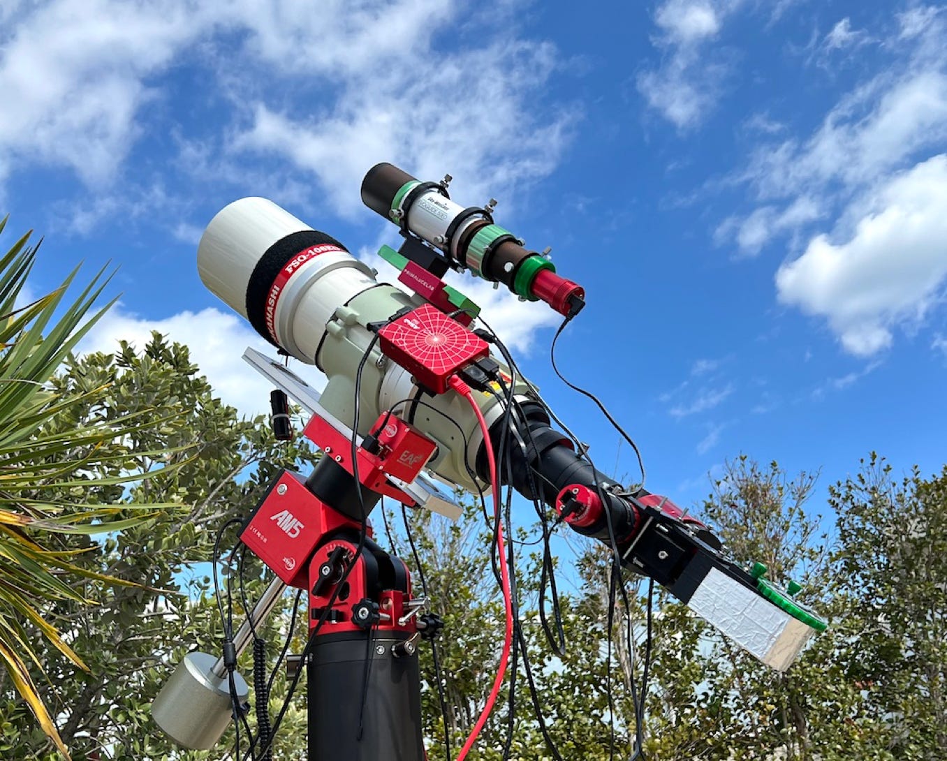
The ASIAir system is used to control the mount, automatically find objects by field recognition and perform autoguiding. The perfect integration of the ZWO system offers an undeniable comfort. Good surprise, even on relatively weak objects in brightness, the device is effective. However, it is assisted in our case by a computer whose task is, independently, to acquire and save the spectra.
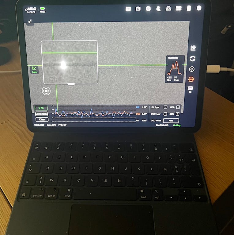
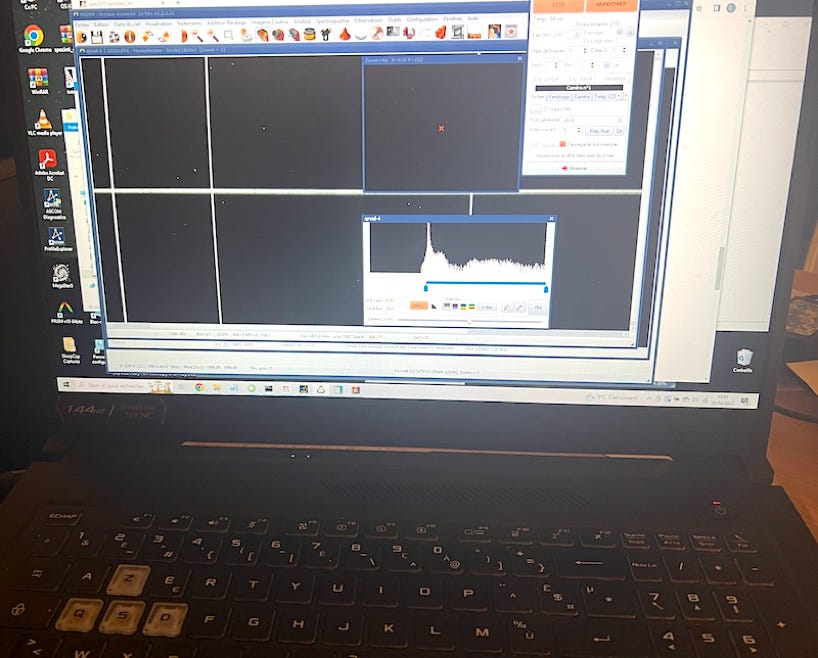
In addition to the high spectral resolution provided by this equipment (Star'Ex HR), we seek to get the maximum to reach targets of low brightness (it is quite natural). We will of course try to optimize all the parameters, such as the focal length for example, as we have just seen, to achieve this objective.
The critical decision concerns the width of the slit. The slit is really the heart of a spectrograph, even if sometimes it is possible to do without it. Too narrow, it prevents the light from entering the spectrograph, too wide, it no longer plays its role in fixing the spectral resolution and spectral calibration. Taking what is indicated in this document, which distills some tips for optimizing its instrument, the optimal slit width in millimeters (for a seeing of 4 seconds of arc) is given by the formula :
w = 0.019 x F
By doing the calculation for our case, we find w = 0.019 x 790 = 0.015 mm
But here, I took the risk of adopting a wider slit than the "standard" value of 15 microns (Shelyak multiple slit), by switching to the "standard" width just above 23 microns. Why am I talking about risk?
First of all, as you can see, I am trying to get as many photons as possible into the spectrograph. A width of 23 microns represents on the sky an angular width in arc seconds that can be calculated with the formula:
Angle = 206300 x w / F
With w = 0.023 mm and F = 790 mm, we find 6 arc seconds. As I often have a very poor seeing of 5 to 6 arc seconds on my site, this is not necessarily an aberrant width, and it is clear that the slit transmission is then relatively high (T slit = 0.84 - see section A4.8). But on the other hand, this causes an area of uncertainty in the positioning of the star in this width, which is likely to generate a spectral calibration error (depending on whether the star is on one edge or the other). Here for example the appearance of a star (here QR Vul, V = 4.75) when it is centered on the slit, which we guess as a narrow horizontal band, here illuminated by the light of the star. This fineness of 23 microns is captured by the ASI290 guidance camera of the Star'Ex system and displayed on the interface of a tablet running the ASIAir software:

The light seen in the center of the slit, as well as the fact that we still see the star in this situation, is explained by the glass support of the slit. The latter reflects about 7% of the incident light towards the guiding camera, a vitreous reflection which is as much loss for the spectrography. It appears that on its width, the slit is not uniformly illuminated, which causes a slight increase in the spectral resolution (a parameter not perfectly stabilized, since it depends on the variation of seeing, which is annoying).
Fortunately, turbulence blurs to some extent this pattern over time, as do guiding errors. Thus, the consequences of using a relatively wide slit do not cause much spectrographic damage, in general.
However, for a "normal" use of the spectrograph, as a safety measure in case of low turbulence, to achieve maximum precision in terms of spectral calibration quality, for radial velocity measurements for example, while bringing a reasonably strong amount of flux into the spectrograph, and for the case in point (a telescope of about 800 mm focal length), I recommend the use of a 19 micron slit with Star'Ex HR rather than the 23 micron slit used in the present demonstration. Typically, switching from a 23 micron slit to a 19 micron slit results in a 15% loss of flux, which is not significant and decisive compared to the spectroscopic gain offered by the 19 micron slit. A small formula useful in passing, which applies to Star'Ex HR when we observe around the Halpha line. If w is the width of the input slit, the width w' of the image of this same slit in the plane of the detector is given by :
w' = 0.602 x w
(the quantity 0.602 is equal to the product of the internal magnification in Star Ex HR (125/80) by the anamorphic factor (0.386)).
If the input slit is 19 microns wide, then its image on the detector is w' = 0.602 x 19 = 11.44 microns. Given the size of the pixels (3.76 microns), the width of the slit is sampled by 11.44 / 3.76 = 3 pixels approximately, which is excellent in spectrography (it is absolutely necessary to exceed with margin the limit value of 2 pixels, a sampling of 2.5 pixels per FWHM being considered as the strict minimum practical).
With a slit of only 15 microns, we find 2.4 pixels per FWHM, which approaches the critical area of undersampling. A 19 micron slit is definitely the right compromise here.
Still on this image, we can note the second parameter to watch very closely: the focus of the star in the slit plane. The sign of a good focus is to see a formed image of the star (in the form of a Gaussian curve) in the center of the slit, but of course very attenuated. Outside the slit, we see the wings of the image of the star that overflow. This is the ideal towards which we must strive. If you are far from this ideal, if the stellar image does not show any shape with a peak, if it overflows the slit while shaking strongly, you have a problem: bad focusing, faulty optics (which is rather rare), high seeing with respect to a slit that is too thin (one aims too far in spectral resolution with respect to what the telescope and the atmosphere can provide - it is necessary to widen the slit then) A trick I give you, which is a way to measure the quality of the focus to the eye: the less the image is defocused, the more it is agitated because of turbulence. Conversely, a focused star forms a "point" and is much more stable.
The quality of the guidance is also important. You should never go below 0.5 seconds of exposure time on the guiding camera, because then you are trying to compensate for the turbulence, which is futile. Rather than shortening the exposure time if the object is bright, reduce the gain of the guiding camera to 0. Ideally, the exposure time in guiding should be at least 1 second, and if possible more, to better integrate the fluctuations of turbulence and thus stabilize the image to be guided.
The defocusing and the weakness of the guidance are by far the main causes of noise in the acquired spectra. These parameters are too often neglected, unfortunately.
Another very important point is to position the center of the stellar image exactly at the center of the slit width. This seems obvious, but the result is far from being acquired, especially when you are a beginner. A shift of 10 to 20% of the position of the star can already cause a significant loss of flux. It is necessary to bring the star to a precise position on the sensor, to about 4 or 5 microns. Not all acquisition software or mounts are capable of doing this, so the operator must be very careful. This is the key to good observation. In the case of the couple AM5 + ASIAir, it seems that the fineness of the slow movements does not allow a precise positioning of the star on the slit when the focal length exceeds 1 meter. ZWO made a mistake by not providing a finer motion to the paddle than the current finest motion (x1), which turns out to be relatively coarse, while the device is capable of guiding to the nearest arc second. This is the main weakness I identified in the ASIAir system, a device rather intended for short focal lengths I find.
In short, the precise positioning of the star on the slit and its sharpness are crucial to make the difference between a good observation and a mediocre one. Try to remember the image above during your observing experience.
We have high ambitions for this observation: we are aiming for a magnitude 12 star with a simple 100 mm refractor and high spectral resolution. You read correctly, magnitude 12!
The target object is the symbiotic star YY Her. We aim at the Halpha line with our spectral resolution of at least R=15000.
Even if the star is of low brightness, there is no problem to point it with the EVOGUIDE 50ED finder thanks to a fast and efficient "plate solving" of the ASIAir. However, ZWO programmers should be cursed to require equatorial coordinates for the day values, while all catalogs provide 2000.0 coordinates. One can clearly feel that the bulk of ZWO users are confined to photographing trivial sky objects, while we, spectroscopists, are interested in the subtleties that this same sky offers - those real well hidden riches - and nothing comes up at ZWO. On the image below, you can see the object in the field of the EVOGUIDE 50ED camera after 10 seconds of exposure. It is important not to miss the target, of course:
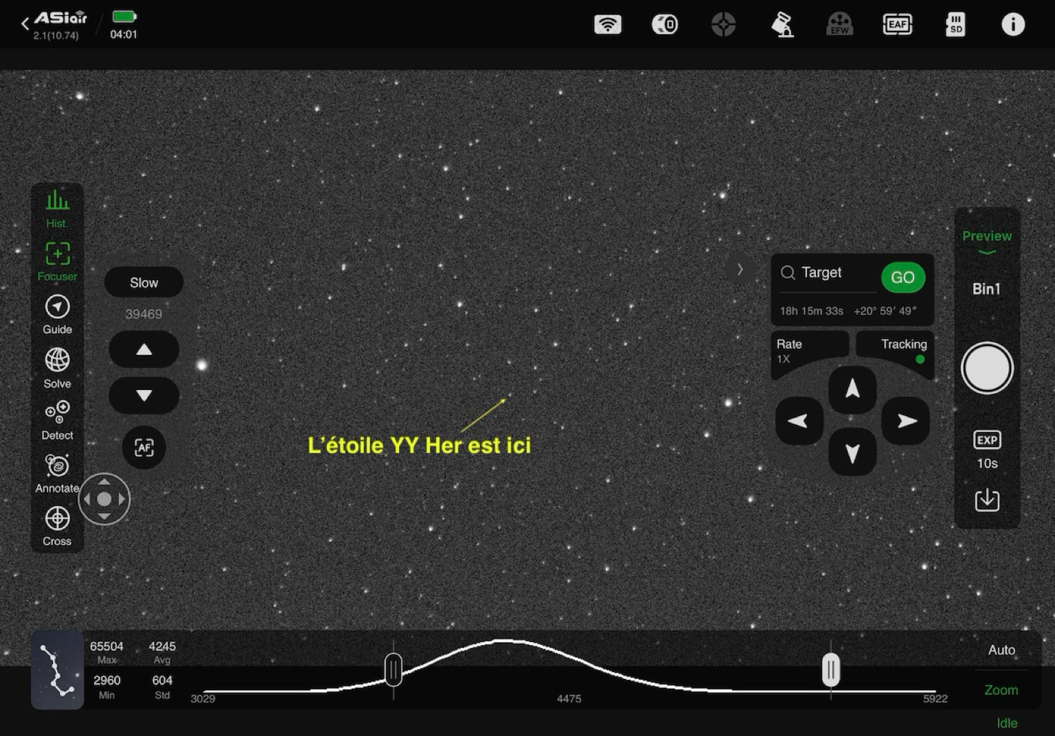
Hereafter, our star in the guiding camera of Star'Ex with an exposure of 30 seconds (it is already visible with an exposure of 10 seconds). It should be noted that I observe in an urban environment, which explains the bright sky in the background. Fortunately, the black slit appears clearly in contrast, which makes it easier to identify its position in the image. This is an advantage of light pollution in this case. ASIAir does not propose a floating reticle to indicate the position of the slit, unlike some good astro software like Prism or PHD Guiding. However, this corresponds to the basic idea of the application, which aims to offer a simple and intuitive interface for the users, but with some regrettable lacks.
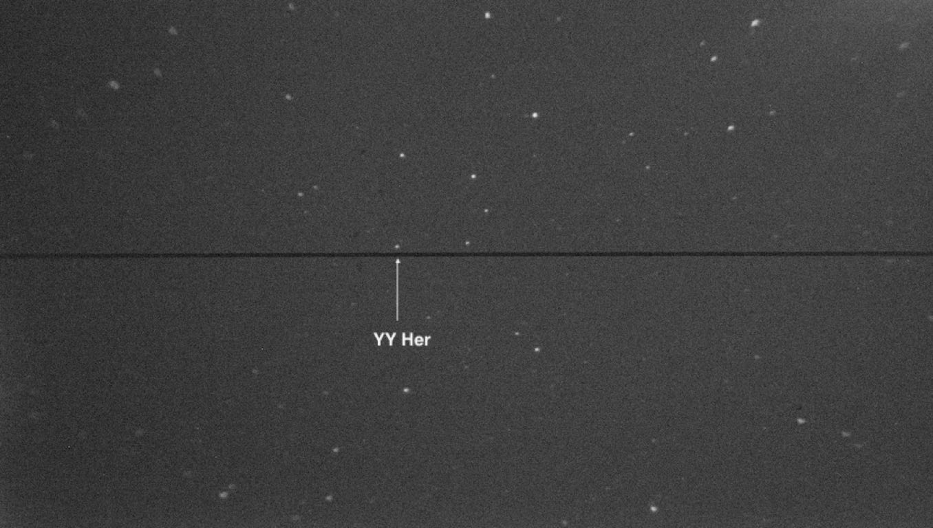
But be careful here, look at this image:
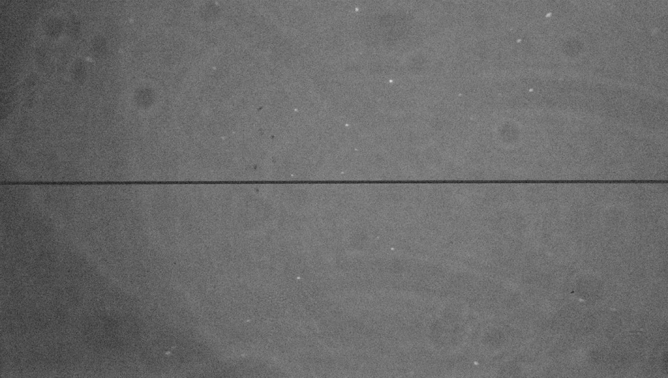
This is the same field and exposure time, but the contrast is much lower, making objects difficult to see. The difference is that in the second case, the calibration system at the entrance of the 100 mm refractor was turned on, with 4 plastic fibers of 2 mm each (see A4.2). This light comes from a neon lamp and acts as a stray light source. Fortunately, we anticipated this and attached a V (green) filter from the BRV system (common bandpass filters, here from Baader) in front of the guiding camera. The goal is of course that the red light from the neon lamp does not reach the detector, being blocked by the filter. In truth, the green broadband filter does not reject all the calibration light, but the residual signal is very weak. Without a colored filter in place (and especially not a red filter), observation would have been impossible, if not complicated. Remember to use this trick of the green color filter in somewhat extreme situations like this; personally, I always keep it in place in front of the guiding camera.
It remains to perform the autoguiding with the tool proposed by ASIAir: the target star is invisible when it is in the slit, so we guide on a star in the field (here, with 3 seconds exposures) :
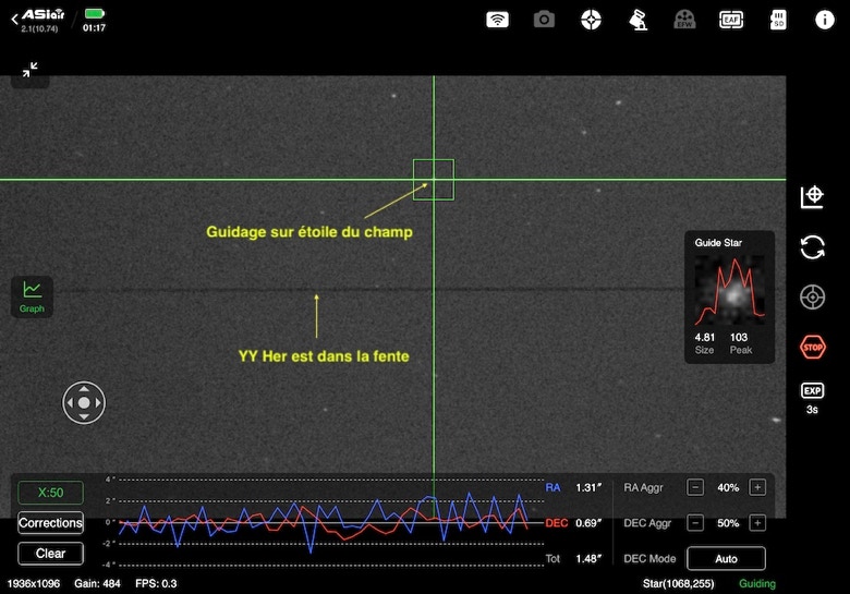
The fourth analog output of the ASIAir box, delivering a 12 V voltage, powers the 4-fiber neon lamp calibration device, via a small 12V-220V converter. During almost all of the 15 minute elementary exposure times required to capture the spectrum of YY Her, the lamp is not powered due to the weakness of the observed star. Only 30 seconds are used to turn on the lateral spectral calibration for each 15-minute exposure, a command that can be executed from a tablet or cell phone. These 30 seconds are enough to print a readable trace of the standard lines in the image:
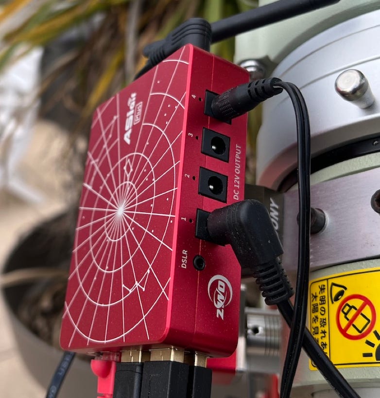
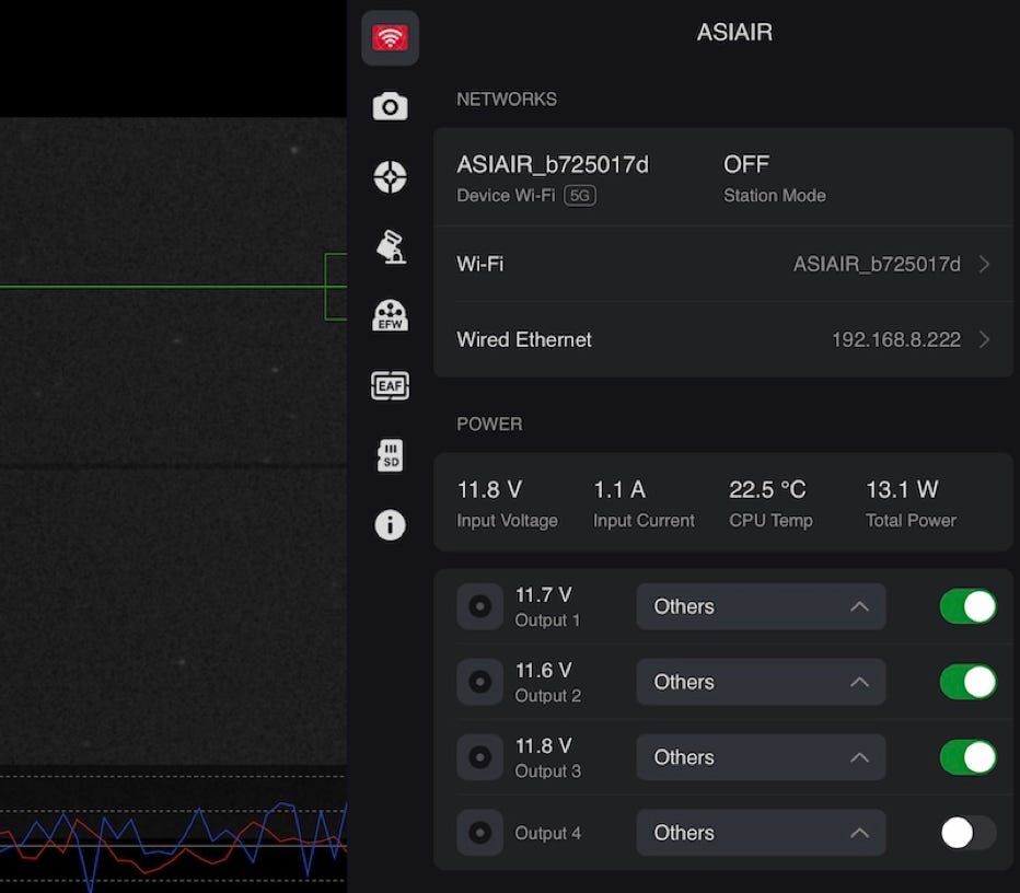
Here is the result obtained on a 15 minutes exposure with an ASI533MM Pro camera cooled to -20°C. In ultraweak spectrography, it is important to expose for a sufficient time to reduce the negative effect of detector noise on the final result.
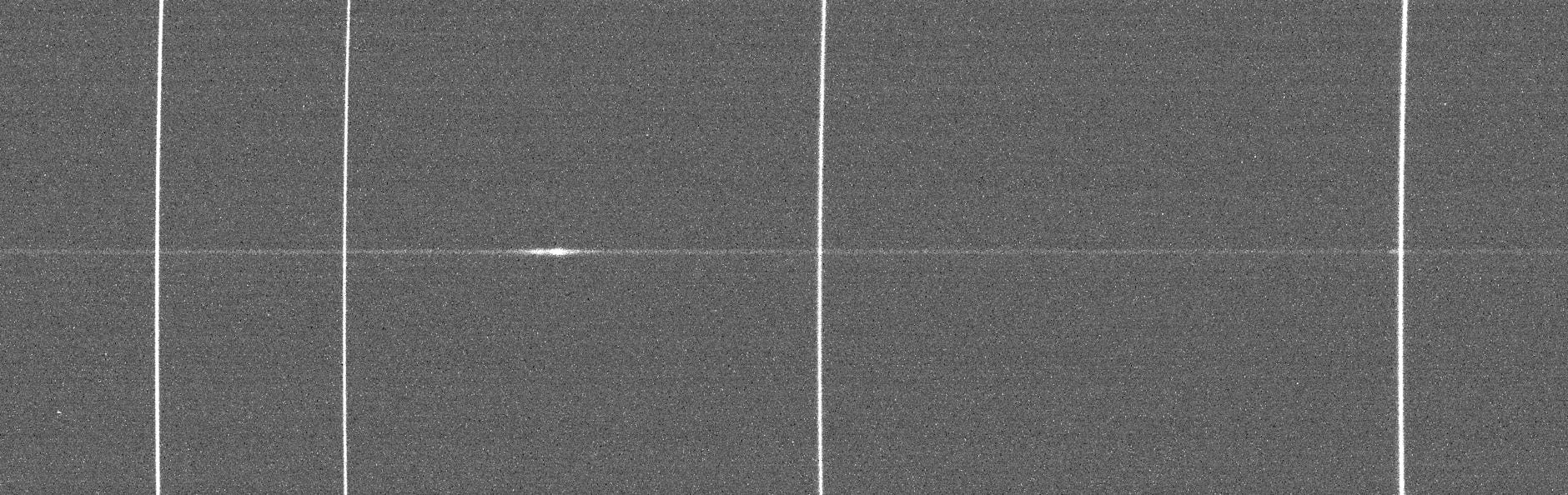
At this stage, three lessons can be learned: (1) the continuum of a magnitude 12 star, with a spectral dispersion of about 0.1 A/pixel, can be detected on a raw image exposed for 15 minutes, which is good news for the future, (2) the calibration lines are present with an intensity consistent with the intensity of the spectrum trace, and (3) a nice line in emission is visible.
It remains to process the ten images of YY Her obtained under the same conditions (2.5 hours of exposure in total). For this, we use specINTI in calibration mode 3 (lateral) with a noise reduction kernel RTS of -3, a Gaussian smoothing parameter of 0.75 (which finally produces a resolving power of R = 15000) and the optimal extraction, which brings here a real visible gain. Here is the final result:
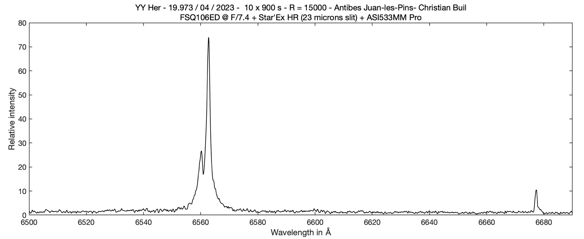
The intensity of the Halpha line in emission is spectacular, about 75 times higher than the continuum level. We can also observe the emission of the He I line at 6678 A, but unfortunately, its profile is degraded by the presence of a neon gas calibration line.
The signal to noise ratio in the continuum is about 8. Thus, we can observe stars of magnitudes 12 at least with a 100 mm refractor in high resolution (R = 15 000). We can see magnitude 13 by accepting a slight degradation of the spectral resolution and on an SNR criterion of 3 or 4. Of course, you have to expose long enough, but it is a classic of spectrography and in fact, it is very simple. It is even possible to work over several nights. By extrapolating, we can consider that the limiting magnitude of a small 72ED telescope operated under similar conditions is of the order of V=11.5 to R = 15000.
The secret ? A good material, not necessarily expensive, well adapted to the objective, a little method and especially, dare!
Note that the observational approach adopted here draws the outline of the spectrographie 2.0.
A4.11: What is the efficiency of my telescope and how to check it?
This is a vast question, which takes us into the intimacy of a spectrograph and optics.
The efficiency of a spectrograph, sometimes called "throughput", is the rate of conversion between the flow of photons reaching the entrance of the telescope and the signal observed at a point of the spectrum, also called "spectral channel".
The calculation is not trivial because the result depends on a very large number of parameters whose value is sometimes imprecise. In the jargon of optics, we speak of the establishment of a "link balance" between the input of the instrument and the output. Despite its inaccuracy (an uncertainty of 10 to 20% is common), the calculation is important in instrumentation to anticipate the performance of a device or detect a malfunction.
I will make here a simplified calculation that will concern only one wavelength of the spectrum, but which applies in the same way for all wavelengths. I will quickly go over some points, but I will still break down the calculation to show the process. You will know more about the functioning of your Star'Ex and what makes its quality and its defects.
The efficiency calculated here is global: it concerns the spectrograph itself, of course, but also the telescope and the detector. I use an example: a Star'Ex LR spectrograph, equipped with a 300 t/mm grating, mounted at the focus of a 150 mm diameter Newton Quattro telescope open at f/4 (SkyWatcher). The acquisition camera is the ZWO model ASI533MM Pro.
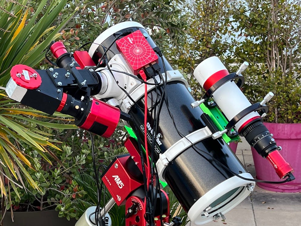
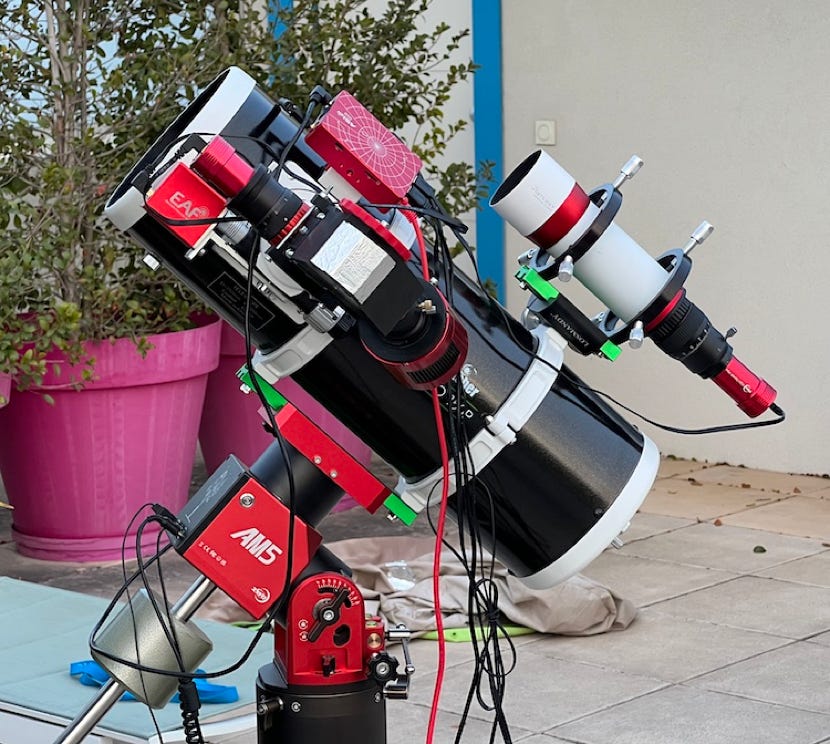
To verify the accuracy of our numerical modeling of the instrument, it is advisable to compare it to a real and concrete measurement. We have therefore chosen to use the star Vega, a bright object visible in the summer sky, considered as a spectrophotometric standard. However, this choice is not optimal, because the brightness of Vega requires the use of very short exposure times to avoid saturating the detector. This increases the sensitivity to turbulence, because their temporal fluctuation is not well averaged. Consequently, the signal of the star varies significantly from one exposure to another. In addition, it is difficult to position such a bright object correctly in the center of a narrow slit.
For more accuracy, it would be preferable to use a less bright star, selected from the CALSPEC standards catalog, for example. This star would be better suited because it would require longer exposure times, thus reducing the sensitivity to turbulence generated by the atmosphere. In addition, the variability of the signal would be reduced, which would facilitate the comparison with numerical modeling.
The value of the photon illumination of Vega is about 1000 photons per square centimeter per second and per angstrom at the Earth level in the green, a value easy to remember. This means that if the width of the band is multiplied by 10 (10 A), the value of this illumination is also multiplied by 10, as well as the area and duration of counting photons.
To avoid the pitfall of the slit, which leads to an inaccurate measurement given the random fluctuations of the optical flow mentioned earlier, we chose a particular measurement strategy. It applies here to Star'Ex but it could also be adopted with an Alpy600 or a Lhires III.
The narrow slit of Star'Ex is replaced here by a slit with two widths. One part of the length of the slot is 23 microns wide (so it's a thin slot), while the other part of this length (less long) is occupied by a 200 microns wide slot (so it's a wide slot, very wide even). The image below is a screenshot of the ASIAir application, showing the shadow of this particular slit on the luminous background of the sky, with in this case, the star Vega positioned at its widest part:
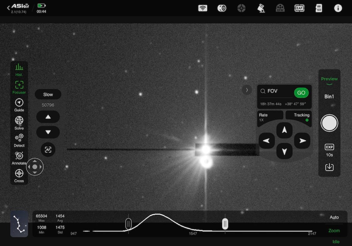
The interest of this arrangement is to make it possible to take a spectrum in two different situations:
- First situation: the star is positioned on the narrow part of the slit to acquire a spectrum in the traditional way. The spectral resolution is then fixed by the width of the slit (thus a fixed resolution, which is important to compare spectra between them). The operator is obliged to position the star at a precise location, which ensures consistency between the spectral calibration of the acquired spectra and standard spectra (spectra of a spectral lamp). The brightness of the sky background is drastically reduced by the fineness of the slit, which allows to observe objects of low brightness, even in town). Finally, the star is well isolated from its neighbors, and there is almost no risk of accidental overlap of spectra.
- Second situation: the star is positioned on the wide part of the slit. In this case, we lose more or less the advantages of an observation with a narrow slit, but we gain others. The positioning of the star is quite loose, which makes observations easier. But above all, we have the guarantee that 100% of the flux focused at the focus of the telescope enters the spectrograph (except for a small attenuation depending on the technology adopted to make the slit - see below). In fact, the slit is much wider than the image of the slit agitated by the seeing, even with force. Another interest, more subtle, but which can be essential, is that the atmospheric chromatism making the stars focused at the focus of the telescope form a mini-spectrum, which lengthens when approaching the horizon, has no impact on the measured spectra. The size of the atmospheric spectrum is much smaller than the width of the wide slit, and so its impact is integrated into average photometry - it is no longer visible. This is a major item of error removed on the continuum shape, which everyone is victim of, sometimes violently (much higher than the error of evaluation of the spectral response proper of the instrument).
One can guess that the spectrophotometric quality, both absolute and relative, is much higher when the spectrum is acquired with the star in the wide part of the slit. I have named this type of slit "photometric slit". The presented model is available from Shelyak. The classic use consists in merging by processing two spectra: the first is made in the narrow part to detail the spectrum, the second, much coarser in terms of details restored, is made in the wide part to find the exact aspect of the continuum of the star. We thus obtain both a spectrum with good spectral resolution, but also another with good radiometric resolution, giving access to the Spectral Energy Distribution (SED in the jargon).
Let's add that the use of a mixed slit helps the use of the spectrograph: to beginners to make their first spectra without the constraint of a sometimes confusing autoguiding, to more experienced observers to focus the image of the star in the slit (the sharpness in width of the spectrum trace is a very good tracer of the quality of the focus, better and simpler than the judgment of the sharpness when the star is in the narrow part of the slit.
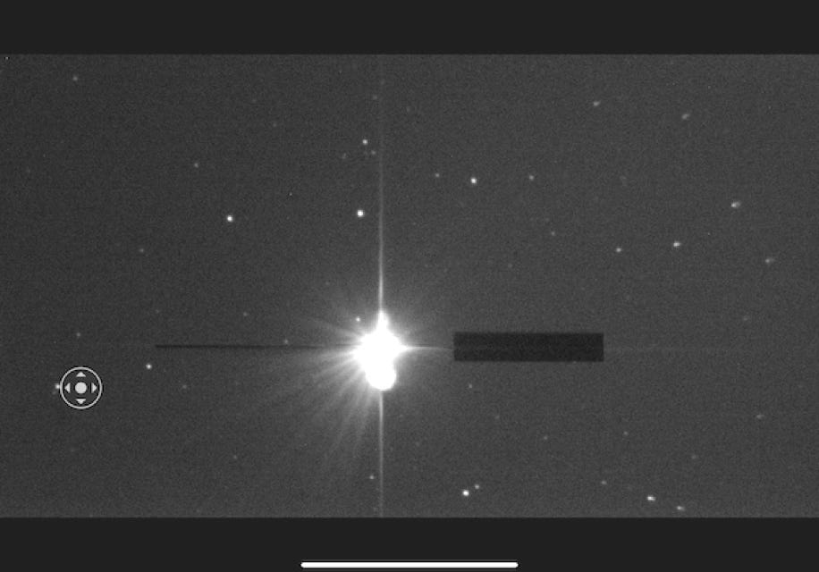
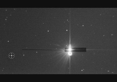
In these views, on the left, the star is positioned in the narrow part of the slit (the image is saturated for the purpose of visualization). We are in spectrographic mode. On the right, the star is in the wide slit, we are in spectrophotometry mode.
Here we use the photometric slit only to help us measure the performance of the Star'Ex LR (outside the slit) by positioning the star in the wide part.
The exposure time is 1.2 seconds, chosen so that no point of the spectrum exceeds the saturation threshold of the detector (65535 apparent ADU). The signal near the 5500 A wavelength is extracted from the spectral profile using the -5 mode proposed by specINTI (see section 11.5, the calculation of the signal in digital counts (ADU) for each column of the detector between two predefined lines - this is a basic binning around the spectrum trace). The sky background signal is subtracted beforehand, as well as the removal of the offset signal and the dark signal if desired in the observation file.
At wavelength 5500 A (approximately), a digital signal of 5.35 x 10^5 ADU is found for 1.2 seconds of exposure. But beware, there is a catch: the AQSI544MM Pro camera operates in 14 bits, while the image is displayed in pseudo 16 bits. The manufacturer artificially multiplies the raw signal by 4 to synthesize a false 16 bits. This will have to be corrected, because the gain of the camera - the conversion rate between the number of ADUs and the number of electrons - is given here for a digitization on 14 bits. Precisely, our camera is operated with a manufacturer's gain (or apparent) of 150, which gives an electronic gain (reciprocal) of 0.59 e-/ADU (value measured by the author). Finally, the signal recorded in number of electrons for an exposure time of 1.2 seconds is estimated at :
S_obs = 5.35 x 10^5 x 0.59 / 4 = 7.89 x 10^4 e-
We must now try to find this value from the numerical modeling of Star'Ex, our famous bond balance.
The precise illumination of Vega at 5500 A above our atmosphere is 1010 photons/s/A/cm^2, which will be noted F = 1010 photons/s/A/cm^2.
Before reaching the telescope, this flow of photons must cross the obstacle of the Earth's atmosphere. This one absorbs the light according to the transparency of the moment (AOD) and the angular height of the star above the horizon. We estimate that this absorption is 0.70 (a value to be noted in the file "_trans_atmo.fits" if you make the complete treatment of the star with specINTI), that we will note T1 = 0.70.
The telescope consists of two mirrors covered with a single layer of aluminum protected. We estimate the reflection coefficient of a mirror to 0.91; for two mirrors, the result is 0.91^2 = 0.83. We will note T2 = 0.83.
The surfaces of the lenses of Star'Ex are covered with simple anti-reflection treatments (MgF2), with a transmission coefficient of 0.985 per side. Since there are two lenses and 4 faces, the transmission for all these lenses is 0.985^4 = 0.94 (the internal absorption of glasses is considered zero at 5500 A). We will note T3 = 0.94.
The internal vignetting in Star'Ex LR, despite the use of a very bright telescope, with an F/D ratio of 4, is considered zero. We note T4 = 1.0.
The slit used, despite being large, still retains some light, because it consists of a thin sheet of glass, one side of which is not treated anti-reflection, hence an estimated optical transmission of 0.96. We note T5 = 0.96.
The diffraction efficiency of the grating of 300 lines/mm is estimated at 65% for the considered wavelength (Richardson documentation). We note T6 = 0.65.
The quantum efficiency of the Sony sensor of the ASI533 pro camera is considered 85% at 5500 A. We note QE = 0.85.
The overall efficiency (including the atmosphere and photon-electron conversion via the quantum yield) is the product of all these terms:
E_global = T1 x T2 x T3 x T4 x T5 x T6 x QE = 0.70 x 0.83 x 0.94 x 1.0 x 0.96 x 0.65 x 0.85 = 0.29
This value; E_global = 0.17 includes the effect of atmospheric transmission. The instrumental throughput is obtained by doing the same product, but without the atmosphere, here a throughput of 0.29 / 0.70 = 0.41, which is very high for this category of instrument.
Taking into account the central obstruction, the collecting surface of the telescope is S = 144 cm² (obstruction of 0.43). The spectral sampling of Star'Ex LR is about d = 1.54 A/pixel with the camera used and finally, the exposure time is Ti = 1.2 second, hence the value of the theoretical signal calculated in number of electrons (e-) for a spectral channel at 5500 A:
S_calculation = F x S x E_global x d x Ti = 1010 x 144 x 0.29 x 1.54 x 1.2 = 7.79 x 10^4 e-
This result should be compared with the measured flux (see above): 7.89 x 10^4 e-. The difference between the observation and the calculation is almost insignificant (largely within the margin of error of this type of calculation and measurement).
It is highly probable that by doing the same experiment with a narrow slit the difference between the observed and the calculated (O-C) is significantly larger, of course to the disadvantage of the observation. The slit selection effect at the entrance of the spectrograph is generally a major item in the binding budget. A loss between 60 and 70% of the flux is quite common in this area. And if the turbulence is strong or the slit guiding is approximate, then it is half of the optical flux that is lost, or even worse.
The spectrograph has a performance that is what it is (very honest in the case of Star'Ex LR), and often there is little choice for telescope selection (in the example taken, the central obstruction is severe, and we saw in section A4.9 that a refractor could give a much clearer image because of the natural transparency of its optics). Finally, the only lever you can act on is the right choice of slit width, a good focus of the telescope, a good guiding, an observing site that gives you some respite from atmospheric turbulence. The acquisition of good spectra is at this price: everything happens at the level of the entrance slit (unless you remove it, as indicated in the answer to question A4.6 of this page).
An advice if the opportunity arises: compare the signal obtained in your spectral profile between an observation of the same object with a slit and without a slit; the result is often edifying... and encourages to do better!
A4.12 : I found an answer concerning the performance of Star Ex "low-resolution", but what about Star Ex "high resolution" used with a refractor?
Indeed, answer A4.11 deals with the efficiency of a Star'Ex LR spectrograph associated with a particularly luminous Newton telescope. The calculation method for a Star'Ex HR spectrograph is quite similar, but of course the numerical values change. The use with a refractor makes another difference.
As always, I will rely on an observation to check what the theoretical calculation says.
The Star'Ex HR spectrograph is characterized by the internal optical configuration "80x125" and by the use of a 2400 lines/mm grating. The associated camera is an ASI533MM Pro. For this test, I also use a photometric slit with two widths: 23 microns and 200 microns. Star'Ex is set on the Halpha line. It is associated with a SkyWatcher EVOSTAR 100ED scope of 100 mm diameter and opened at F/9. This aperture ratio allows to operate Star'Ex directly at the focus, without significant internal vignetting and thus without having to use a Barlow lens, which simplifies the system. This refractor, because of its low price, its diameter, its lightness and its rather favorable F/D ratio for spectrography, proves to be a good companion of Star'Ex. An EAF focuser is added and the whole set is mounted on an AM5, the whole driven by the ASIAir system (except for the acquisition of the spectra which is done here via Cyril Cavadore's Prism software)
Our target is the faithful star Vega, a spectrophotometric standard well placed for the northern hemisphere and bright.
The screenshot below shows the image of the star Vega positioned in the widened part of the slit (200 microns). The strange appearance of the diffraction is due to the spectral calibration system placed in front of the objective (a 2 mm optical fiber and its support):
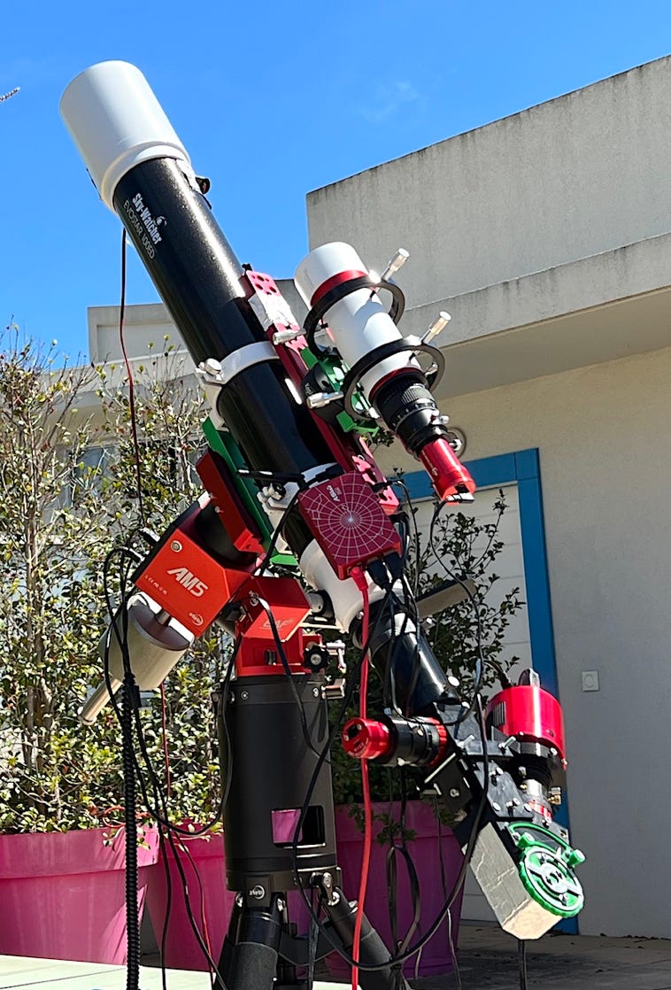
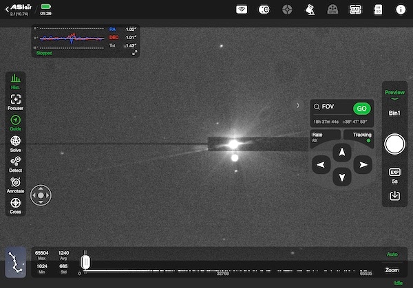
Here is the characteristic aspect of a spectral image. The spectrum presented corresponds to the star Alpha Draconis after an exposure of 600 seconds. The size of the image acquired with the Prism software is limited to the surface of the sensor considered as useful at the time of the observation. This avoids cluttering the hard disk with too large image files. We left a piece of the wide slit in the lower part of the image to allow spectrophotometric measurements. The alpha star Draconis is placed in the thin part of the slit. We can also observe the lines of the calibration neon in superposition (this is the lateral mode):
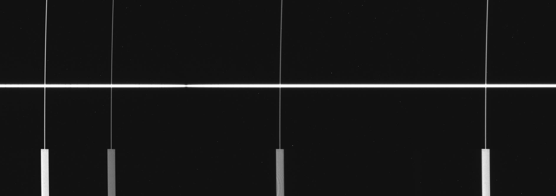
After summing the spectra of the Vega star exposed for 90 seconds each, for a total of 540 seconds, a raw signal of 2.18 x 10^6 digital account units (ADU) at a wavelength of 6630 A was found, using the -5 extraction mode. This signal is the sum of the intensities of the corresponding sensor column in the spectrum image. Before this, the offset and dark signal were subtracted. According to the indications of the answer A4.11, it is necessary to convert this intensity on 16 bits in a dynamic of 14 bits and to convert it in number of electrons:
S_obs = 2.18 x 10^6 x 0.59 / 4 = 3.21 x 10^4 e-
For the simulation, the following numerical values were selected:
- Atmospheric transmission for the angular elevation of the star: T1 = 0.85
- Transmission of the refractor, with a multi-layer anti-reflection at 0.995 for the 4 faces of the objective of the 100ED: T2 = 0.98
- Internal transmission of the objectives of the spectrograph (4 faces treated MgF2): T3 = 0,94
- Optical vignetting at F/9 : T4 = 0.95
- Transmission of the slit substrate : T5 = 0,96
- Diffraction efficiency of the grating at 6630 A : T6 = 0.32
- Quantum efficiency of the detector at 6630 A: QE = 0.54
The overall efficiency is obtained by multiplying all these values:
E_global = T1 x T2 x T3 x T4 x T5 x T6 x QE = 0.85 x 0.98 x 0.94 x 0.95 x 0.96 x 0.32 x 0.54 = 0.123
To calculate the photonic signal sent by Vega at the wavelength of 6630 A, we recovered the spectrum of Vega out of atmosphere in the CALSPEC database accessible from ISIS or SpecINTI (adaptation of the database available on the site: https://www.stsci.edu/hst/instrumentation/reference-data-for-calibration-and-tools/astronomical-catalogs/calspec). The unit of energy in this spectrum is erg/cm2/s/A. At wavelength 6630 A, the illumination induced by Vega above the Earth's atmosphere is E = 1.84 x 10^-9 erg/cm2/s/A. The flux expressed in number of photons/cm2/s/A is obtained from the formula :
F = lambda x F / 1.99 x 10^-8 , with lambda in angstroms,
or here,
F = 6630 x 1.84 x 10^-9 / 1.99 x 10^-8 = 613 photons/cm2/s/A
The collecting area of the entrance refractor objective is S = 78.5 cm^2 (formula pi x D^2 / 4), the spectral sampling of Star'Ex HR around Halpha is d = 0.10 A, the exposure time is Ti = 540 seconds, hence the value of the theoretical signal in electrons calculated for a spectral channel at 6630 A :
S_calculation = F x S x E_global x d x Ti = 613 x 78.5 x 0.123 x 0.10 x 540 = 7.79 x 10^4 e- = 3.20 x 10^4 e-
As previously stated, the result of the observational measurement is 3.21 x 10^4 electrons. This agreement between the observation and the calculation is not a coincidence. It is obtained by manually adjusting one of the parameters of the numerical model of the instrument: the grating diffraction efficiency (T6). It is common in this type of numerical model to have one or more adjustment variables, especially for parameters whose characteristics are poorly known or difficult to measure in the conditions of use of the components concerned.
In our calculation, we set the value of T6 to 32%, while the manufacturer of the array indicates an efficiency of 45% at 6630 A for unpolarized light. To match the observations and the model, we were forced to consider a grating about 30% less efficient than what is predicted by the supplier of this optical part. This lower performance may be due to the fact that we are not working at Littrow incidence in Star'Ex (i.e. when the diffraction angle of the light rays is identical to the angle of incidence of these same rays on the grating). It is shown that when we move away from this Littrow incidence, the diffraction efficiency of the grating decreases significantly, depending on the type of grating used.
In the case of a holographic grating, which operates in a complex regime, called "electromagnetic", we consider plausible an efficiency of 32% in the red part of the spectrum. However, the situation improves in the blue part of the spectrum, because we then approach the Littrow incidence. In fact, Star'Ex HR shows a higher efficiency in the blue part of the spectrum compared to the red part.
This analysis allows us to understand how the value of the parameters that influence the level of signal recorded for a given object is established, excluding effects such as seeing, guiding errors or inaccurate focusing of the images. We also note that the clean efficiency of the instrumental set used (telescope + spectrograph), known as "throughput", is about 15% in the red. Although this may seem low, it is common to see this efficiency in instrumental spectrography at high spectral resolution. This does not prevent obtaining very good spectra, simply by adjusting the exposure time.