specINTI & specINTI Editor
9 : Low resolution spectrography
Low-resolution spectrography is attractive, because it allows to capture the whole visible spectrum at once, rather than a portion, always more abstract. Unfortunately, and probably counter-intuitively, low-resolution spectrography is difficult to practice. The pressure is on both the hardware and the user. On the hardware, because low resolution is similar to wide-field imaging, which requires a complex optical system. The large spectral range covered, by definition, also implies a demanding chromaticity management. For the user, because it is not easy to perform a quality spectral calibration over a wide range of wavelengths, while simultaneously, the search for the true continuum of the star is quite perilous. The message is clear: if you are new to spectrography, choose high spectral resolution rather than low resolution.
After this warning, let's see how to reduce low resolution spectra with specINTI.
9.1 : The state of the art
Our support for this description is a set of raw images as they come out of the telescope and can be downloaded from this link: starex234.zip
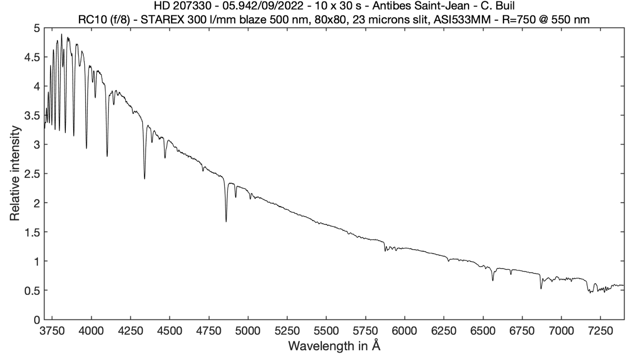
Unzip this archive into a folder. We assume here that the path of the folder is "e:/starex234", but you are free to choose the location and the name. Included are raw data acquired with a 10-inch (D=254 mm) Richey-Chretien telescope open at f/8 (RC10 f/8), with a Star’Ex spectrograph at the focus of it in a configuration that includes a 23 micron wide slit, a 300 line/mm grating, the 80 mm focal length camera lens, and a CMOS ASI533MM camera. Those familiar with Star'Ex will surely have recognized a configuration called "low spectral resolution", allowing to capture the whole visible spectrum in a single image. The observatory is located near the city of Antibes in the south of France, that is to say in an urban site near the sea.
The observation concerns on the one hand, the star HD207330 (quite bright, magnitude 4.2, and spectral type B3III) and on the other hand, the star SS Cyg (cataclysmic type, at magnitude 12 at the time of acquisition). You will find 10 raw images of the spectrum of HD207330, and 8 images of the spectrum of the star SS Cyg, as well as additional files (offset, dark, flat-field, spectral lamp).
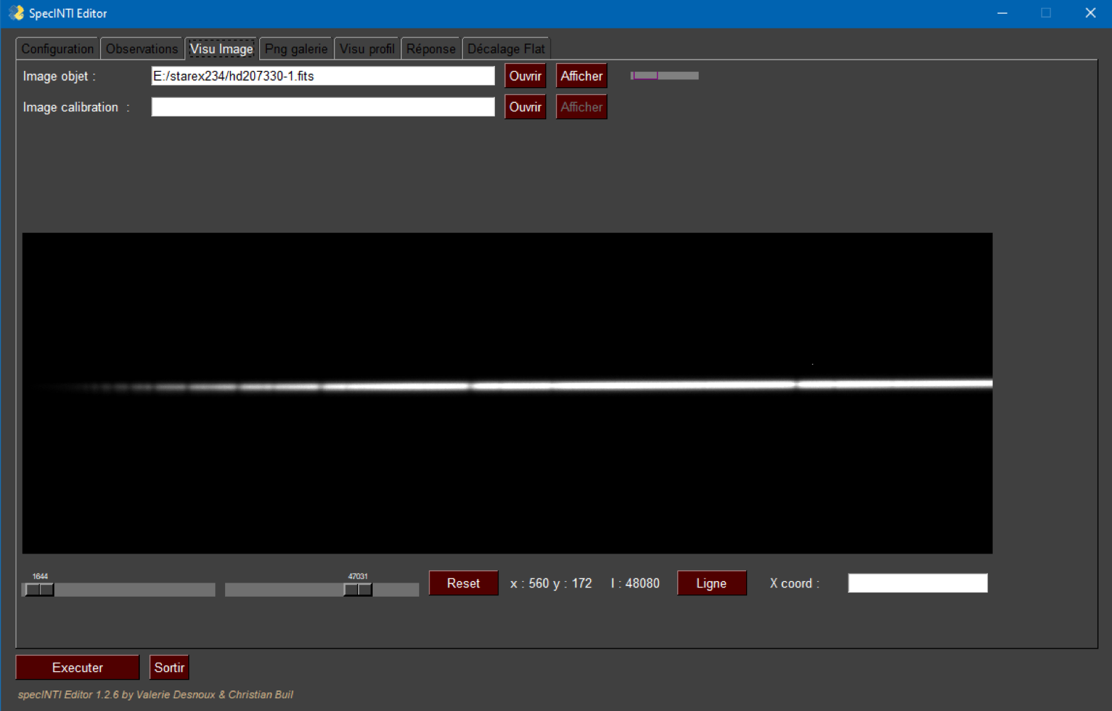
Here is the look of a raw image of the star Hd207330-1.fits (an extract of the blue side):
Or the image of a spectral calibration spectrum - here from a neon lamp:
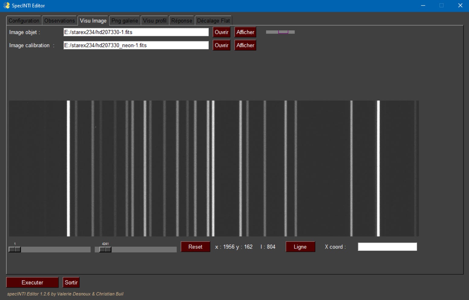
This kind of barcode, in negative, shows the fine lines produced by the neon lamp waved in front of the telescope aperture just after the observation of the star HD207330. These emission lines will help us later to calibrate the wavelength spectrum.
Note: as already recommended; all data are acquired in 1x1 binning. In addition, remember that it is useless to work on a complete image because the spectral image of the star is only a thin line on the sensor. We will therefore crop the images from the acquisition (cropping) to save space on the hard disk and later, accelerate the calculations. Here the window isolated in the full frame of the sensor is 3008 x 331 pixels. We used the Prism software for the acquisition, which performs this type of cropping in a safe and reproducible way. Generally once we have chosen the windowing parameters, we never change them for a given instrumental configuration. You will then have a bank of calibration images that you can re-use at will. This is time saved.
9.2 : A small tour through the observation file
We will begin by extracting the spectrum of the star HD207330. We exploit for this the 10 elementary acquisitions made to increase the famous Signal to Noise Ratio (or SNR).
It is considered that you have read section 5.1 of this documentation, which lays the foundations of the concept of "observation file".
After opening the "Observations" tab, remember to first update the path of the observation directory, or working directory, for example: "e:/starex234/ ".
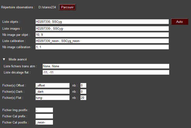
Also check that your prefix and postfix are correct with respect to the way you name the raw image files. For example here :
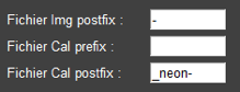
In the "Object list" field, enter the name of the object to be processed, here HD207330: this is its catalog name. It is also the generic name used to name image files, which is not a coincidence and the interest will appear immediately. Click on the "Auto" button at the top of the tab and specINTI Editor will fill in all the other fields for you, saving you work and avoiding errors.
specINTI Editor has found the name of your raw images and enters the result of the root name "HD207330-" in the "Image list" field. The number of images in the sequence was also automatically entered in the "No. of images per object" field. The program has also detected the presence of an associated calibration image, whose root name is " HD207330_neon- ". The importance of naming your image files correctly! If you had more than one calibration image, the software would have seen it. Here there is only one.
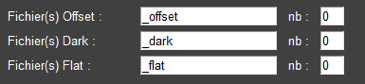
Check that the fields " Offset ", " Dark ", " Flat ", contain the name " none ".
You can also fill in the "Observations" tab from an observation file already present in the image directory. Just double click on the name "obs_hd2073390_demo1.yaml" in the list on the right. But it is best to fill in the tab yourself to get a good feel for how to proceed.
It is perfectly possible to save this observation file under the name of your choice, in the working directory, via the "Save" button at the bottom of the tab.
The description of the observation is minimal, but sufficient for a first test. Here is what the "Observations" tab looks like at this stage:
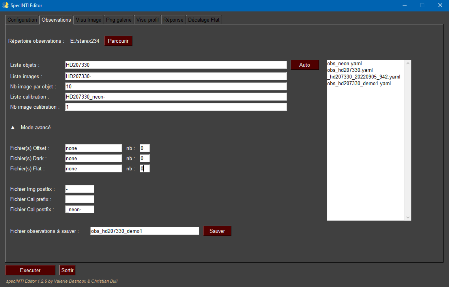
You are then in a really minimalist processing configuration ("obs_hd2073390_demo1.yaml" in the working folder). Indeed you have not provided any name for the offset, dark, flat-field pre-processing images. You are perfectly entitled to reduce your spectra in this way (note the use of "none" to indicate that we do not have the reference images in question).
Although this is not recommended, we will for the moment remain in this situation to judge the consequences of this choice.
9.3 : A little tour through the configuration file
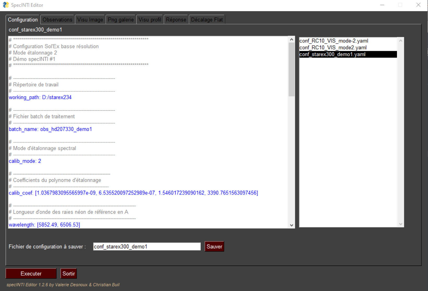
Open the "Configuration" tab and instead of entering all the parameters by hand, just use the predefined configuration file "conf_starex300_demo1.yaml" by double clicking on its name in the list on the right. Here is the result:
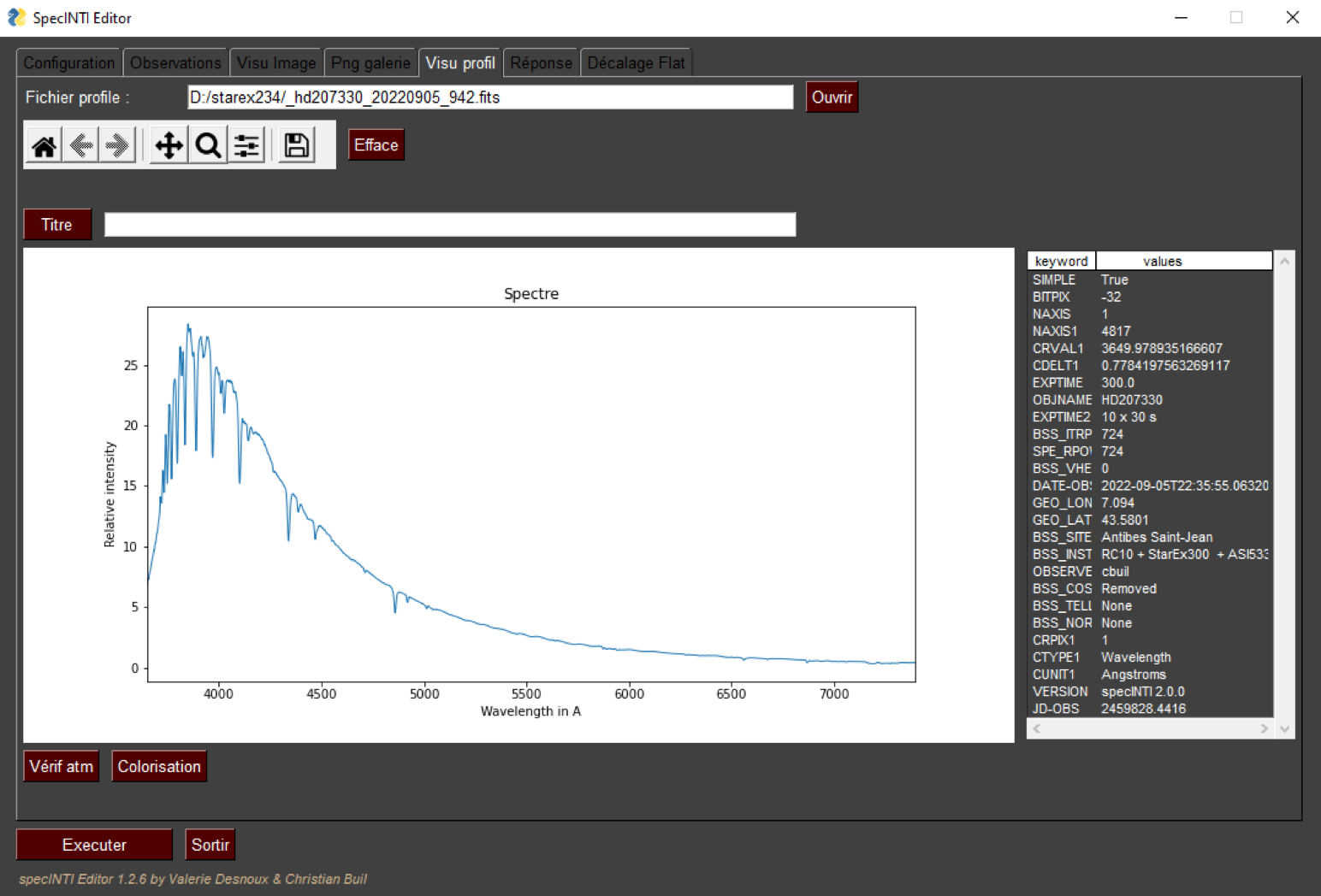
Let's launch a first treatment by clicking on the "Run" button. After a few moments, the spectrum profile appears in a thumbnail. It now also exists in the working folder as a FITS file, with the name "_hd207330_20220905_942.fits". Let's display the contents of this file in a large format from the "Profile view" tab:
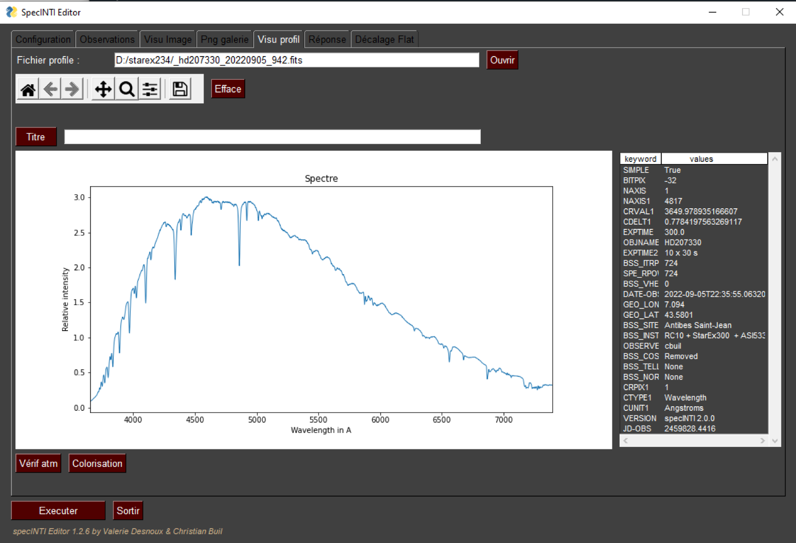
We have here the (very rough) appearance of a hot star spectrum observed in low resolution from 3700 A in the blue, up to 7400 A, at the edge of the infrared. The promise of the wide spectral range is well kept.
Unfortunately, this spectrum is far from resembling the expected theoretical shape. The profile as we have just extracted it is marred by many defects. In particular, we have skipped the pre-processing step, which is classic by the way, consisting in subtracting from the raw images the offset signal, the dark signal and dividing by the flat-field to eliminate a maximum of defects in the response of the detector and the optical train. In short, it is a sloppy job!
But before improving the situation, we suggest that you take a look at the contents of the configuration file as is, here is the complete listing:
# ********************************************************************
# Sol'Ex low resolution configuration
# Calibration mode 2
# Demo specINTI #1
# ********************************************************************
# ----------------------------------------------------------------
# Working directory
# ----------------------------------------------------------------
working_path: D:/starex234
# ----------------------------------------------------------------
# Processing batch file
# ----------------------------------------------------------------
batch_name: obs_hd207330_demo1
# ----------------------------------------------------------------
# Spectral calibration mode
# ----------------------------------------------------------------
calib_mode: 2
# -------------------------------------------------------------
# Coefficients of the calibration polynomial
# ------------------------------------------------------------
calib_coef: [1.0367983095565997e-09, 6.535520097252989e-07, 1.546017239090162, 3390.7651563097456]
# -----------------------------------------------------------------------------
# Wavelength of the reference neon lines in A
# -----------------------------------------------------------------------------
wavelength: [5852.49, 6506.53]
# ----------------------------------------------------------------------------
# Position of the neon reference lines in pixels
# ----------------------------------------------------------------------------
line_pos: [1580, 2000]
# ---------------------------------------------------------------------------------
# Width of the reference line search area
# ---------------------------------------------------------------------------------
search_wide: 20
# ----------------------------------------------------------------
# Binning width
# ----------------------------------------------------------------
bin_size: 22
# ----------------------------------------------------------------
# Sky background calculation areas
# ----------------------------------------------------------------
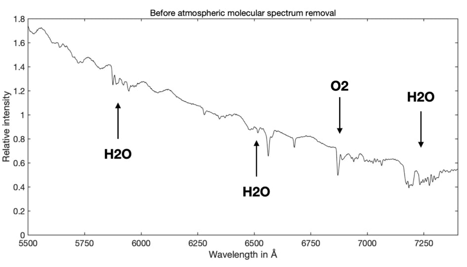
sky: [120, 20, 20, 120]
# -------------------------------------------------------------------
# x-boundaries for geometric measurements
# ------------------------------------------------------------------
xlimit: [500, 2000]
# ----------------------------------------------------------------
# Normalization zone to the unit in A
# ----------------------------------------------------------------
norm_wave: [6400, 6420]
# ----------------------------------------------------------------
# Profile cropping area
# ----------------------------------------------------------------
crop_wave: [3650, 7400]
# ----------------------------------------------------------------
# Longitude of the observation place
# ----------------------------------------------------------------
Longitude: 7.0940
# ----------------------------------------------------------------
# Latitude of the observation site
# ----------------------------------------------------------------
Latitude: 43.5801
# ----------------------------------------------------------------
# Altitude of the observation point in meters
# ----------------------------------------------------------------
Altitude: 40
# ----------------------------------------------------------------
# Observation site
# ----------------------------------------------------------------
Site: Antibes Saint-Jean
# ----------------------------------------------------------------
# Description of the instrument
# ----------------------------------------------------------------
Inst: RC10 + StarEx300 + ASI533MM
# ----------------------------------------------------------------
# Observer
# ----------------------------------------------------------------
Observer: cbuil
# ------------------------------------------------------------------------
# FITS file extension (0 -> .fits, 1 - > fit)
# ------------------------------------------------------------------------
file_extension: 0
You should be in familiar territory if you have already gone through section 5.5.
Note the value 2 given to the "calib_mode" parameter. Remember that this number specifies the spectral calibration procedure to be adopted to perform the processing. The possible options are described in section 10. Mode 2 means that the spectral dispersion law (the relationship between the rank of pixels in the spectrum and the wavelength) is already evaluated as a polynomial function. If lambda is the wavelength, and x a pixel rank number in the spectrum, the polynomial function performs the operation: lambda = f(x). The way to evaluate the coefficients of the spectral dispersion polynomial will be described later.
The parameter "calib_coef" gathers the terms of the spectral calibration polynomial, those of the famous calibration function, which is imposed here:
calib_coef: [1.0367983095565997e-09, 6.535520097252989e-07, 1.546017239090162, 3390.7651563097456]
This is a polynomial of degree 3. This degree fixes in some way the fineness of fit of the spectral law. The degree 3 is appropriate here given the fact that we work in low spectral resolution and given the distribution of reference lines that will allow us later to establish the value of these coefficients. In a more classical form, more mathematical, here is how it presents our polynomial (by rounding the values):
Lambda = 1.03680e-09 X^3 + 6.53552e-07 X^2 + 1.54602 X + 3390.765
The values of the parameters "wavelength" and "line_pos" indicate respectively the wavelength of lines produced by the neon lamp of calibration and the approximate position of these lines in the image in pixels and along the horizontal axis (axis of dispersion). specINTI will use this information to adjust the first term of the calibration polynomial (see "calib_coef"), the so-called "constant" term, to take into account a possible spectral shift between the time the polynomial was evaluated and the time the observation is performed. This wavelength correction is the basis of calibration mode #2. All other terms of the polynomial are assumed to be stable and remain unchanged (they could have been calculated well before the observation or after). In our example, we chose two lines at coordinates x = 1580 and x = 2000 (you can find them in the image HD207330_neon.fits). specINTI will average these two measurements (you could very well define one line or 10). You have a tolerance on the X position accuracy. This tolerance is set by the "search_wide" parameter. In the example, it is +/-10 pixels, which is generous (be careful not to set too large a tolerance, as specINTI may confuse neighboring lines). If you don't define "search_wide", the default tolerance value is +/-25 pixels.
9.4 : A little tour through the console
Remember that specINTI delivers a certain amount of information in the output window (be careful, it can be hidden by the main window) while the program is running. Here is an example of this processing log:
-------------------------------------------------
specINTI 2.0.0
Path = D:/starex234\
-------------------------------------------------
Observation file: D:/starex234\obs_hd207330_demo1.yaml
****************************************************
Target: HD207330
****************************************************
Target processing...
..........
Total exposure time = 300.0 seconds
Computed mean Y = 177
Processing calibration...
$$$$$ -> _step3
..........
Tilt correction...
Computed tilt angle = -0.329
..........
Slant correction...
Computed slant angle = 0.002
..........
Sky substraction...
Profile standard extraction...
Evaluate lines position...
Predefined calibration function + computed shift...
Calibration coefficients:
1.0367983095565997e-09, 6.535520097252989e-07, 1.546017239090162, 3390.7651563097456
Resampling...
Mean spectral shift = 15.850 A
FWHM = 5.12 pixels
Dispersion = 1.5460 A/pixel
Resolution power = 724 @ 5732 A
Compute stacking...
Cropping...
Normalize...
SIMPLE = 'T '
BITPIX = -32
NAXIS1 = 4818
CRVAL1 = 3649.978935166607
CDELT1 = 0.7784197563269117
BZERO = 0
BSCALE = 1
EXPTIME = 300.0
OBJNAME = 'HD207330'
EXPTIME2= '10 x 30 s'
BSS_ITRP= 724
SPE_RPOW= 724
BSS_VHEL= 0
DATE-OBS= '2022-09-05T22:35:55.063200'
GEO_LONG= 7.094
GEO_LAT = 43.5801
BSS_SITE= 'Antibes Saint-Jean'
BSS_INST= 'RC10 + StarEx300 + ASI533MM'
OBSERVER= 'cbuil '
BSS_COSM= 'Removed '
BSS_TELL= 'None '
BSS_NORM= 'None '
CRPIX1 = 1
CTYPE1 = 'Wavelength'
CUNIT1 = 'Angstroms'
VERSION = 'specINTI 2.0.0'
JD-OBS = '2459828.4416'
----------------------------------------------------
Output files names:
D:/starex234\_hd207330_20220905_942.fits
D:/starex234\_hd207330_20220905_942.png
D:/starex234\_hd207330_20220905_942_2D.fits
D:/starex234\_hd207330_20220905_942.yaml
D:/starex234\_hd207330_20220905_942_log.txt
----------------------------------------------------
End of the processing.
able to analyze it with specialized programs like VisualSpec, ISIS, SpAudace, etc.
The file _hd207330_20220905_942_2D.fits is an image strongly resembling the 2D images of the spectrum of the star HD207330, except that it is the sum of the 10 raw images, pre-processed, with the sky background removed, geometrically corrected (for example the tilt angle is now zero) and recentered along the vertical axis
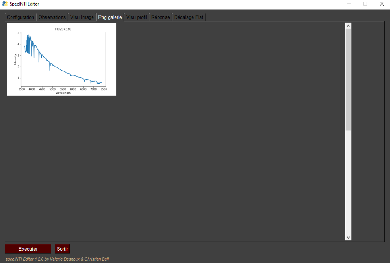
The _hd207330_20220905_942.png file is a PNG graphic thumbnail image of the star profile (it is a so-called "Quick-Look" version, useful for making a small illustrated base of profiles or for communication).
The file _hd207330_20220905_942.yaml is a copy of the configuration file used to process the object. This copy will be precious if after a day, a month or a year, you want to reprocess your images identically (just copy this YAML file in the subdirectory "_configuration" of the specINTI installation directory).
You will also find a file _hd207330_20220905_942_log.txt which contains an excerpt from the "log" we are describing.
Remember that the log can be more extensive if you add the following line to the configuration file:
cherck_mode: 1
9.5 : Offset, dark, flat-field and so on
The previous pre-processing of the spectral images of the star HD207330 is far from being done in the rules of art. In particular, it does not respect one of the foundations of astronomical image processing, which is the removal of biases induced by the detector, among others. Remember that before becoming spectra in the form of curves (spectral profiles), the data acquired with a spectrograph are indeed images, so you will not be disoriented if you come from astronomical photography.
Examine the contents of the working folder associated with this demonstration. You will find:
- An image of the offset signal, o-1.fits. Reminder: the offset images are obtained by closing the telescope aperture and posing for a very short time (0.1 seconds for example, or less). You can also be in a dark room, the telescope is not necessary.
- A series of 15 images of the dark signal, exposed here 900 seconds each, named n900-1; n900-2, ... n900-15. The dark images (or of the dark signal, also called thermal) are made by closing the aperture of the telescope and posing at least as long as the longest exposure time practiced on the stars. During the day, you can use a stratagem by making the darks after having put the spectrograph with its camera in a refrigerator compartment to simulate the coolness of the night and by passing the cables through the doorway. specINTI knows perfectly well how to digitally adjust the exposure time of all your images for a coherent processing with the exposure time of your "dark" master. So, if you have acquired spectral images with a 180 second exposure, there is no need to make 180 second darks, as those exposed for 900 seconds will be perfectly suitable for processing, the software will do the right thing. It is however important that the temperature of the sensor is always the same (-12°C for the data of this demonstration).
- A sequence of 15 flat-field images, named tung-1, ... tung-20. These images were taken during the day, on a table, following the procedure described in section 5.4.
One of the tasks of the software is to subtract the offset signal and the thermal signal (image of the dark signal from which the offset signal has been removed) from all the raw images, then divide the result by the flat-field image (itself corrected for offset and dark). This division allows to remove a good part of the spectral response of the instrument, response that is unfortunately not uniform along the spectrum. When we say "response" we mean "sensitivity" of a point of your detector to the flow of light rays that arrive at the entrance of the telescope.
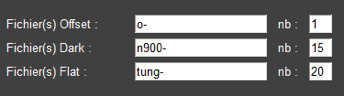
To tell specINTI to apply the treatment using the offset, dark, flat-fied calibration images, you have to fill in the corresponding fields in the "Observations" tab (use the "Auto" button so that specINTI finds the number of images for you):
Restart the process by clicking on the "Run" button (without doing anything else, it is useless, because specINTI Editor automatically saves your changes). The result is quite different from the previous one:
This profile is much more similar to what we can expect from a hot star like HD 207330 (lots of blue, not too much red).
However, the profile is still disturbed by the "spectral response of the instrument", that is to say the way the instrument as a whole (telescope + spectrograph + detector) modifies the true signal of the star as a function of the wavelength. This distortion comes from the optical transmission which colors the luminous flux which crosses it, from the quantum yield of the detector which varies with the wavelength, etc. To put things in order, we will have to establish this famous instrumental response, then rectify the distorted form of the spectrum by dividing it by this response. This is often the most difficult part when you start in spectrography, and especially in low resolution spectrography.
Now let's make two small adjustments, one in the observation file, the other in the configuration file.
The more experienced among you may have noticed an anomaly in the pre-processing done previously. We have only one image of the signal (o-1.fits). This is very little to hope to minimize the noise in the master offset image, because we do not have the possibility to average independent acquisitions of the offset signal. But this choice is voluntary, because with recent Sony CMOS sensors (for example that of the ASI533MM camera), the offset signal, apart from the noise, is almost similar for all pixels. We might as well consider the master offset image as a perfectly uniform image, which can be synthesized by an elementary calculation, and where the noise is zero. To do this we will insert a function in the configuration file, following a principle explained in section 5. Just add the following line in the configuration file, wherever you want:
_img_make_offset: [o-1, _offset]
The function "_img_make_offset" analyzes the image "o-1" by calculating its average intensity, then synthesizes an artificial image by giving all pixels the average intensity previously calculated. This synthetic image is saved in the working folder automatically under the name "_offset". The image in question is very similar to the real offset, but without any noise. Start the program by clicking the "Run" button. It stops automatically when the function has completed its calculation. The "_offset" image is now on your disk. Finally, delete the line of the function.
In the observation file you can now write (the master images _dark and _flat having been calculated when the program was first run):
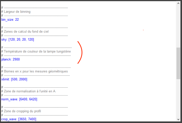
La seconde retouche, qui concerne cette fois le fichier de configuration, consiste à y ajouter le paramètre «planck», qui permet de tenir compte de la température de couleurs de la lampe tungstène utilisée pour réaliser le flat-field :
# Tungsten lamp temperature
planck: 2900
To see the result, simply click the "Run" button after making changes in the configuration file:
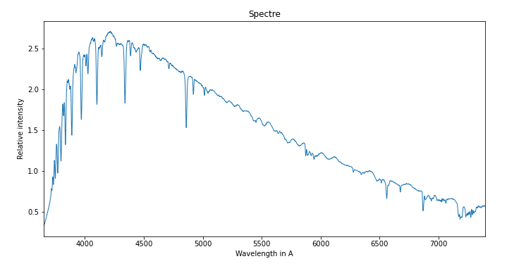
The lines in the ultraviolet part of the spectrum are better perceived. However, the calculated spectrum is not yet satisfactory. In particular, the kind of more or less periodic oscillations that can be seen in the red are not a very good sign, because they are certainly not natural (the continuum of such a star is actually quite smooth). We will have to remedy this!
9.6 : The correction of the atmospheric transmission
While we are in the configuration file, let's calculate the spectrum outside the atmosphere by adding the "corr_atmo" parameter (see section 5.8.2):
# ———————————————————————————
# Atmospheric transmission correction
# ———————————————————————————
corr_atmo: 0.13
Hereafter, the aspect of the atmospheric transmission thus calculated as a function of the wavelength (assign the value 1 to the parameter "check_mode" to have this curve). It appears that the absorption of the atmosphere is severe in the blue part of the spectrum (more than half of the signal outside the atmosphere is lost):
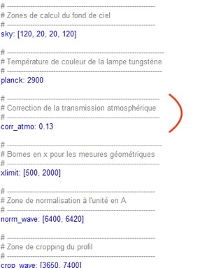
Here is the shape of the spectral profile of the star before the correction of the atmospheric transmission (left), and after correction (spectrum outside the atmosphere, right):
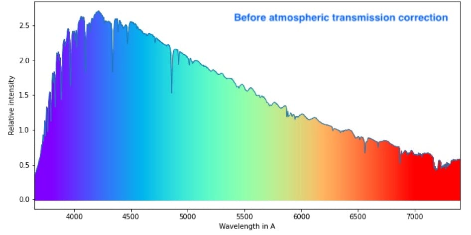
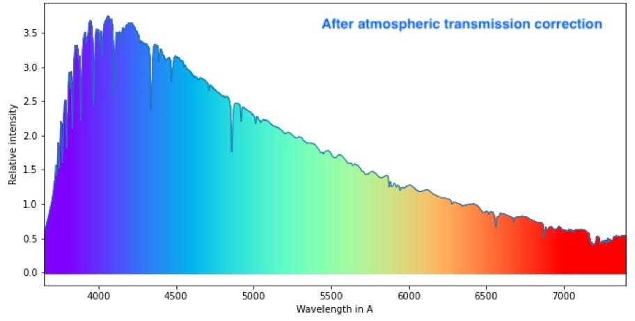
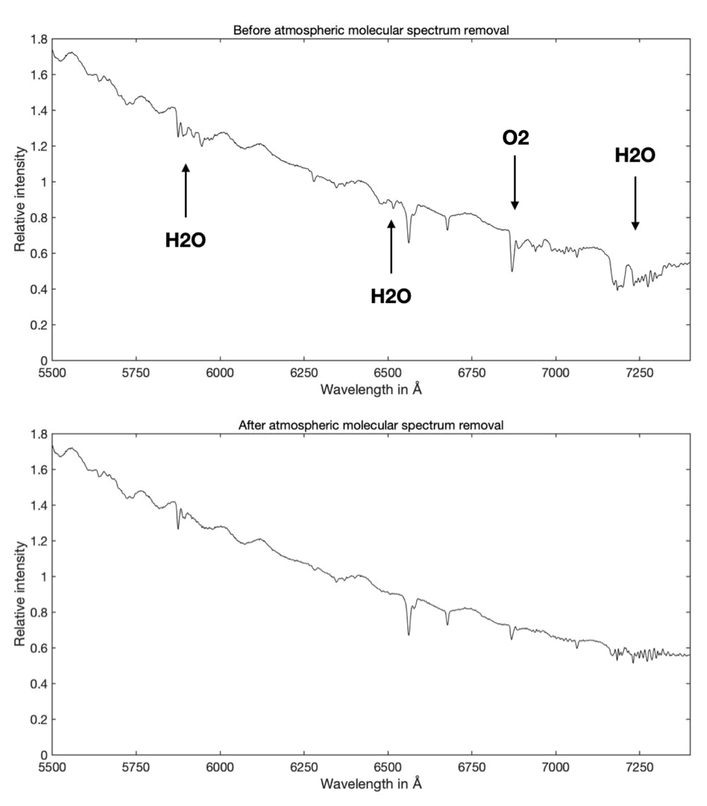
Tip: it is discussed in section 5.8.4 how the spectral profile is made by the diffuse absorption of the Earth's atmosphere, but also by the molecular absorption, and how the latter can be taken into account to evaluate a more accurate out-of-atmosphere spectrum of the star. Let's go back to this procedure (optional, especially since it is relatively complex under specINTI), noting first that the H2O and O2 molecules leave a very visible trace even in the spectra acquired in low spectral resolution :
We will use the file "_molecular_30mm.fits", present in the database "atmo_molecular", that we invited you to download in section 5, to try to erase the trace of molecular lines in the spectrum of the star H D207330 :
1- Copy the file " _molecular_30mm.fits" in your working folder (in the example D:\starex\)
2 - From the "Observations" tab of specINTI, pull down the "Advanced mode" menu.
3 - In the field "List of trans atm files", write the name of the atmospheric transmission file from the ESO model (without specifying the .fits extension):
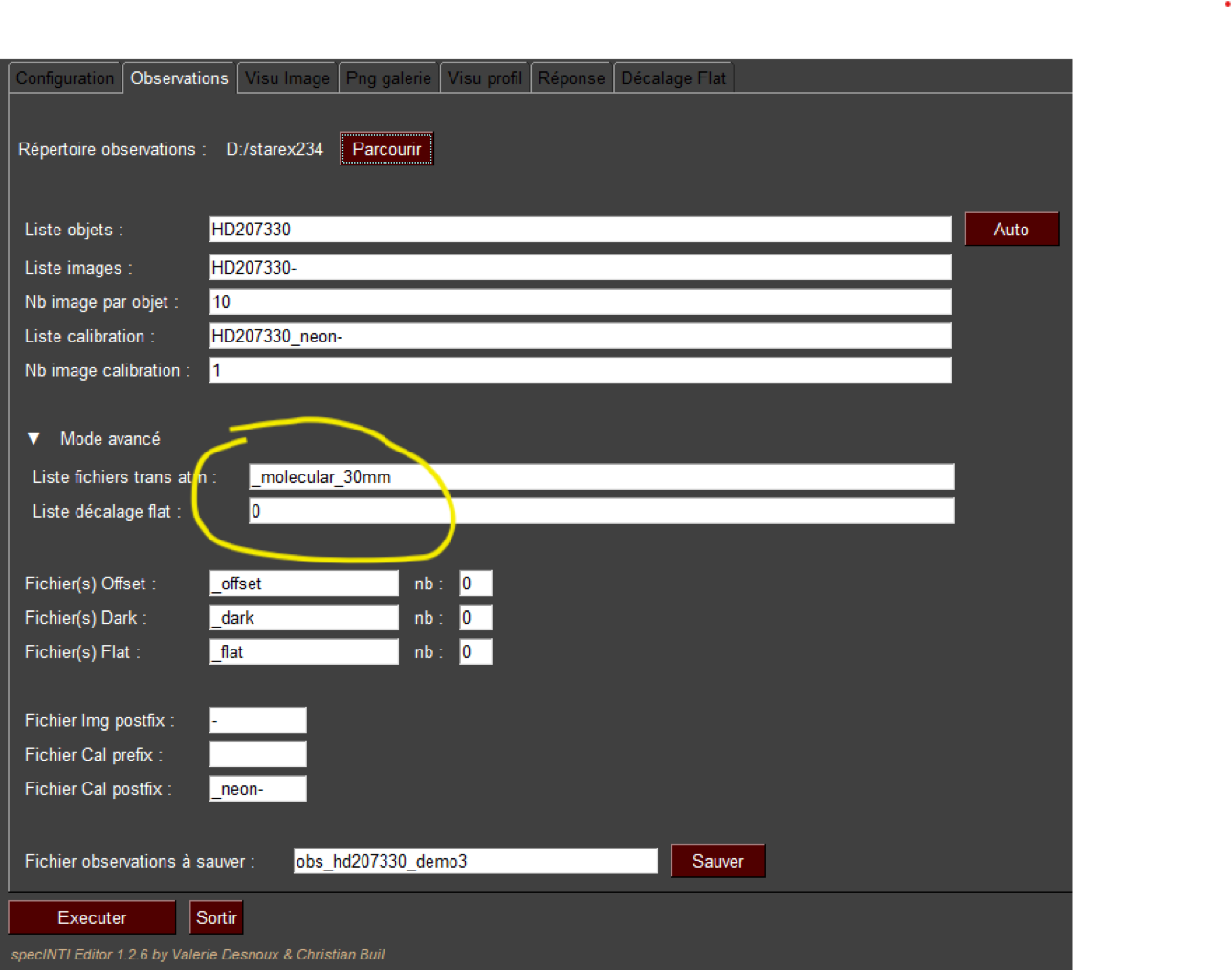
4 - In the current configuration file, add the "atmo_blur" parameter with the value 25 :
atmo_blur: 25
This value is the one found by successive tests to drive the synthetic spectrum of the atmosphere to resolution of our spectrograph.
5 - Launch the treatment by clicking on the button "Execute".
In the profile extracts below, before the removal of telluric lines and after :
9.7 : Wavelength calibration
In section 7.3 we simply indicated that we were using a dispersion polynomial to calibrate the spectrum in wavelengths. In our case it is written :
Lambda = x^3 * C3 + x^2 * C2, x * C1 + C0
With,
C3 = 1.03680e-09
C2 = 6.53552e-07
C1 = 1.54601
C0 = 3390.7651
But where do the coefficients of this function come from, how are the values estimated?
To answer these questions we must have a spectrum with a set of lines whose wavelength is well known (lambda0) and whose position x can be measured in a 2D image of the spectrum in question. From these pairs (lambda0, x), if possible numerous and well distributed to reduce the margin of error, we exploit a mathematical tool capable of passing the best polynomial function (f()) among the measured pairs (method known as "least squares"), such as :
Lambda = f(x)
Note: the technique consists in minimizing the quadratic difference (lambda0 - lambda)^2, between the real apparent wavelengths (or also called "observed") and those calculated with the polynomial (we say "calculated"), it is the O-C.
So, to find the coefficients of the polynomial, you must select a series of pairs (lambda0, x) from the spectrum of a standard lamp with emission lines, in our case a discharge lamp containing neon gas.
Our approach is particular for the shooting of the calibration image. It takes place in two steps:
(1) a first shot outside the telescope, on a table, which concerns only the spectrograph. It is used to evaluate the terms of the polynomial, quietly, detaching from the night of observation. This measurement is generally done only once, as long as the spectrograph is not significantly disturbed.
(2) a second shot, which is made on the telescope, in parallel with the observations on the astronomical targets. This one is only used to readjust the term C0 of the polynomial (constant term) in order to refresh it for the conditions of the observation. The value of this term is affected to the first order by the mechanical bending and thermo-elastic deformations, while the other terms of the polynomial are very little affected (in our instrument the true constants are the terms C1, C2, C3).
For the first benchmark shot, the layout is very simple:
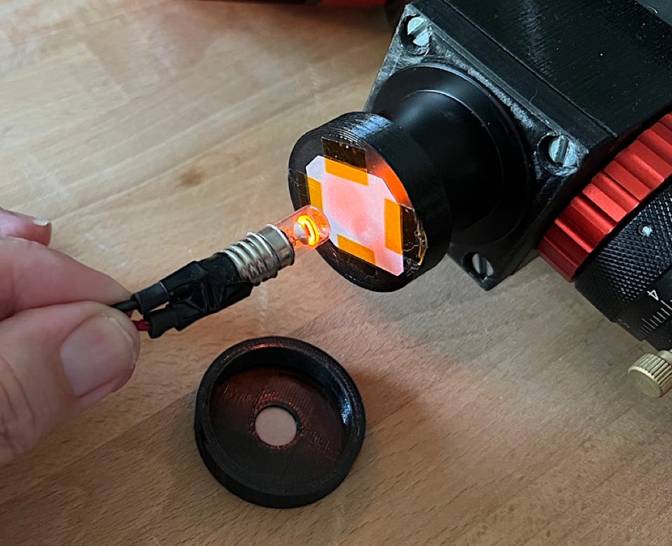
The source is a neon night light with an E10 base (available from Conrad, see this link), which is positioned in front of a diaphragm covered with a diffuser (tracing paper). This setup is similar to the one described in section 5.4. The method of calculating the diameter of the diaphragm is also the same. The diaphragm is made here in 3D printing and mounted at the end of a 31.75 mm slider (for example).
The source is bright and the exposure time is short, about one second. Unfortunately, it is classic with a neon source the most immediately visible lines are located in the red part of the spectrum. By taking care not to saturate the detector by the choice of exposure time (here 0.5 seconds), here is what it gives in the context of our demonstration:

In fact, the lines are concentrated in the right part of the image, that is to say in the red, and nothing in the blue part. This situation is disastrous when it is necessary to adjust a polynomial that is supposed to calibrate all the wavelengths of the explored spectral range (it is possible to interpolate between two lines, while extrapolation with a polynomial, where there is no more information, is risky). You will find this image in the directory of the observation night under the name "tung_neon-1.fits", and you can see for yourself by displaying its contents.
Note: the name of this file starts with "tung" because the images were taken after the flat-field images on the table.
In reality, the situation is not as bad as all that, as a proof, let's look at a second image of the calibration lamp on the table, called "tung_neon-2.fits" (also present in the working folder), exposed this time for 30 seconds, so much more than the first one:
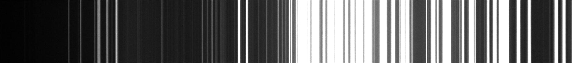
The lines located on the red side are considerably saturated, but good surprise, the presence of lines is also revealed in the green, blue and even ultraviolet parts of the spectrum. These lines will allow us to evaluate a true dispersion polynomial adapted to the low resolution. Unfortunately, the lines on the red side are now saturated because of the long exposure time, and this part of the spectrum is therefore not usable, a priori. Certainly, by playing with the exposure time, we get a relatively uniform distribution of the calibration lines, but the information is diluted in two images, while specINTI accepts only one image to calculate the terms of the polynomial.
The solution to this difficulty is to merge our exposed 0.5 second and 30 second calibration images into a single image, making sure that no line is saturated (precise measurement of the position of a saturated line is indeed impossible). We will use a technique well known in photography, known as "high dynamic range", or HDR (High Dynamic Range). This is how it is possible, in photography, to combine images of the same scene made with different exposure times to unblur the dark parts, while detailing the strong lights.
With specINT, this merging is calculated by writing a single line in the configuration file, the name of the "_img_merge" function, whose syntax is :
_img_merge: [image1, image2, threshold, imageHDR]
with :
- image1, the image of the calibration source realized with the time t1 ;
- image2, the image of the source realized with the time t2 ;
- threshold, a level of intensity in the most exposed image from which it is considered that the saturation threshold is reached;
- imageHDR: the result of the fusion of the two starting images.
As far as the threshold is concerned, if the image is coded on 16 bits, we can consider using the value 65535 (= 16^2 - 1). But it is wise to take a value a little lower than this theoretical maximum, for example a threshold level of 60000 ADU will be perfect in most situations.
Note: the images that come from an ASI533MM camera are actually coded on 14 bits, but the manufacturer artificially multiplies the intensities of all pixels by 4 to simulate a 16-bit image. This is a small deception.
For our application, you write the following line in the configuration file, wherever you like, and then do "Run":
_img_merge: [tung_neon-1, tung_neon-2, 60000, neon_HDR-1]
You can also write a specific configuration file for this function ("conf_make_HDR.yaml" in the distribution):
# *************************************************************************
# Merge two images of the same scene into one HDR image
# *************************************************************************
# ----------------------------------------------------------------
# Working directory
# ----------------------------------------------------------------
working_path: D:/starex234
# --------------------------------------------------------------
# Synthesis of an average image
# --------------------------------------------------------------
_img_merge: [tung_neon-1, tung_neon-2, 60000, neon_HDR-1]
Note: remember that only one function can be found in the configuration file at a time. If there is already one present, delete it, or add a "#" in front of it to make it a comment.
Display the result image "neon_HDR-1" from the "Image View" tab, you will see that it is an HDR image, which shows both low lights (with a good SNR) and high lights (without saturation).
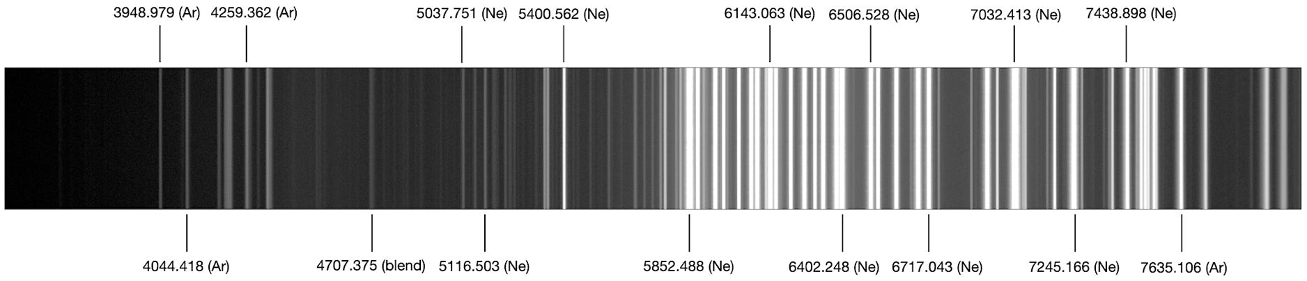
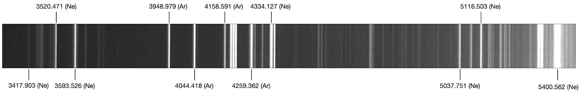
The following document allows you to locate a number of lines that can be used to calculate the dispersion law of our Star'Ex spectrograph on table (here it is a logarithmic display of the image "neon_HDR-1"). The wavelengths are taken from an atlas of many spectral sources that we have compiled, and which can be downloaded at this address:
http://www.astrosurf.com/buil/specinti/Atlas_Spectral_Lamps.pdf
Note: perhaps you wonder why these images of the lamp are not obtained directly on the telescope? The reason is that it would take far too long exposure times to capture the faint lines, so during the nights of observation, which are always too short, there are better things to do than acquire calibration images.
We are now in a situation to find the pairs (lambda0, x). To do this, in the image "neon_HDR-1" locate the position x (horizontal) of some lines that we know the wavelength, using the annotated figure above. For example, the line of wavelength 5400.562 A is found at position x = 1299 (you have a tolerance of several pixels, do not worry - the result will not change if you read x = 1296, for example). So we have a pair (5400.562, 1299). Proceed in the same way for other lines.
Reminder: from the "Image view" tab, to obtain the coordinates of a point in the image, position the mouse pointer on it, then left click.
The elements of each pair are separated in two lists, one for the wavelengths, the other for the coordinates in the image. They are values of the respective parameters "wavelength" and "line_pos". For our example, here is what we have established :
wavelength: [3948.979, 4044.418, 5037.751, 5116.590, 5400.562, 5852.488, 6143.063, 6402.248, 6506.528, 6717.043, 7032.413, 7245.166, 7438.898, 7635.106]
line_pos: [362, 424, 1065, 1116, 1299, 1590, 1776, 1943, 2010, 2145, 2347, 2483, 2606, 2730]
Notes: both lists must contain the same number of elements (specINTI warns you if they don't). There must of course be a correspondence between them (for example, in row number 6, we find our couple (5400.562, 1299)). The establishment of these two lists is relatively tedious, you must not make a mistake. Keep them in a corner for reuse, so you don't have to redo the work.
How to manage these two lists in order to adjust the parameters of a polynomial of a certain degree (here 3) passing through all these pairs of
specINTI offers a special tool which is activated by choosing as calibration mode (the parameter "calib_mode"), the value -2. You have read correctly, it is the value -2 and not 2. In this way, specINTI performs a classical pre-processing on an emission spectrum image, measures precisely the position of the lines whose approximate position is provided by the "line_pos" parameter, calculates the terms of the dispersion polynomial and stops the work at this point.
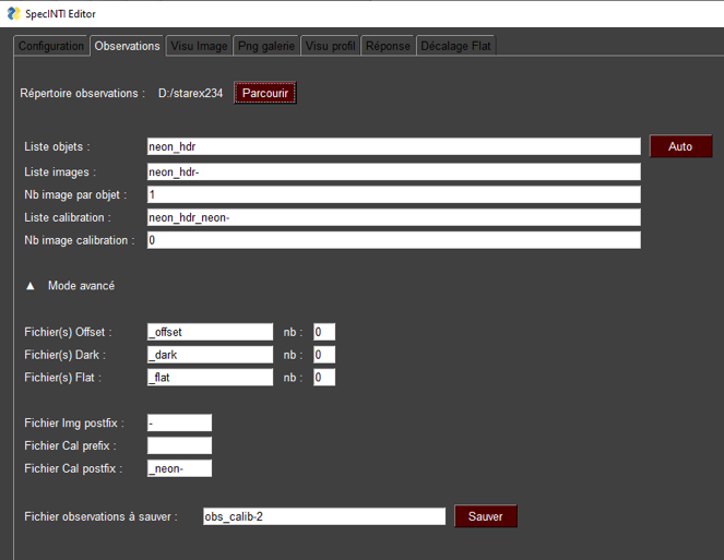
In our situation, the spectral image to be processed is "neon_HDR-1", hence the corresponding observation file, which you name "obs_calib-2" (for example):
The configuration file is presented as follows (you have a copy in the "_configuration" directory under the name "conf_starex300_mode-2.yaml", which saves you typing everything):
# ********************************************************************
# Sol'Ex low resolution configuration
# Calibration mode -2
# Search for the dispersion polynomial from
# an emission line spectrum
# ********************************************************************
# ----------------------------------------------------------------
# Working directory
# ----------------------------------------------------------------
working_path: D:/starex234
# ----------------------------------------------------------------
# Processing batch file
# ----------------------------------------------------------------
batch_name: obs_calib-2
# ----------------------------------------------------------------
# Spectral calibration mode
# ----------------------------------------------------------------
calib_mode: -2
# -----------------------------------------------------------------------------
# Order of the dispersion polynomial to evaluate
# -----------------------------------------------------------------------------
poly_order: 3
# --------------------------------------------------------
# Wavelengths of the standard lines
# -------------------------------------------------------
wavelength: [3948.979, 4044.418, 4707.375, 5037.751, 5116.590, 5400.562, 5852.488, 6143.063, 6402.248, 6506.528, 6717.043, 7032.413, 7245.166, 7438.898, 7635.106]
# -------------------------------------------------------------------------
# Pixel coordinates of the lines in the image
# -------------------------------------------------------------------------
line_pos: [362, 424, 851, 1065, 1116, 1299, 1590, 1776, 1943, 2010, 2145, 2347, 2483, 2606, 2730]
# ---------------------------------------------------------------------------------------------
# Typical vertical coordinate of the spectrum trace of the star
# --------------------------------------------------------------------------------------------
posy: 177
# ----------------------------------------------------------------
# Binning width
# ----------------------------------------------------------------
bin_size: 30
# ---------------------------------------------------------------------------------------
# Width of the search area of the reference lines
# ----------------------------------------------------------------------------------------
search_wide: 10
This YAML file is relatively short. We indicate of course the path of the working folder. Then comes the name of the observation file to use. We specify that the calibration mode is number -2 ("calib_mode" parameter).
The "poly_order" parameter allows you to specify the degree of the polynomial to be adjusted by the least squares method, here the value 3. It is very rare to have to go as far as degree 4, because under the guise of making a more rigorous calculation from a mathematical point of view, this fineness of adjustment takes us away from the actual calibration law when the points to be adjusted are distributed in a non-uniform manner.
The "posy" parameter takes as its value the vertical coordinate (y) of the trace of the approximate spectra in the 2D images (read this value with the mouse pointer, to within a few pixels).
We already know the parameter "bin_size", the height of the agglomeration zone of the signal in the digital 2D images in order to build the spectral profile. Here this width is chosen to be 30 pixels, a typical and rather generous value, in order to obtain a signal to noise ratio.
Finally, "search_wide" specifies the tolerance in pixels for the search for lines from the approximate positions indicated in "pos_line". Here the value is 10 pixels to avoid pollution from lines close to those selected.
Here is the "log" file when running specINTI with this set of parameters:
-------------------------------------------------
specINTI 2.0.0
Path = D:/starex234\
-------------------------------------------------
Observation file: D:/starex234\obs_calib-2.yaml
****************************************************
Target: neon_hdr
****************************************************
Offset:D:/starex234\_offset.fits
Dark:D:/starex234\_dark.fits
Flat-field:D:/starex234\_flat.fits
Target processing...
.
Dark coefficient = 0.033
Total exposure time = 30.0 seconds
Predefined Y = 177
.
.
Slant correction...
Computed slant angle = 0.045
.
Evaluate lines position...
3948.979, 4044.418, 4259.362, 5037.751, 5116.59, 5400.562, 5852.488, 6143.063, 6402.248, 6506.528, 6717.043, 7032.413, 7245.166, 7438.898, 7948.176
----------------
362.23140702118303, 424.29871200599337, 563.1984397309055, 1064.4572726716287, 1115.6126789484579, 1298.550894001235, 1589.0483427917736, 1775.7111261669618, 1942.1253806505647, 2009.0621250549345, 2144.0574956788487, 2346.009322244964, 2482.0270406386467, 2605.632873655251, 2928.8439061486642
----------------
Calibration function...
calib_coef: [1.6185745216759765e-09, -3.193823703854025e-06, 1.5529347323253762, 3387.685356134384]
O-C: [ 0.665 -0.173 -0.659 0.251 -0.29 -0.294 0.239 0.379 0.317 0.226
0.067 -0.228 -0.452 -0.545 0.495]
Root Mean Square Error = 0.3912 A
FWHM = 4.80 pixels
Dispersion = 1.5567 A/pixel
Resolution power = 796 @ 5940 A
End.
Among the many pieces of information returned, we find the terms of the polynomial searched :
calib_coef: [1.6185745216759765e-09, -3.193823703854025e-06, 1.5529347323253762, 3387.685356134384]
You can copy this line as is into the configuration file that is used to process your spectra (in calibration mode 2 for example).
The "log" also provides the difference in angstroms between the Observed lengths (those from the catalog) and the Calculated lines (those from the polynomial), and this for all the specified lines. This is the O-C, useful to identify anomalies (erroneous numerical values for example). The RMS (Root Mean Square) is a parameter that gives a more synthetic view of this difference. It is worth here 0.39 A (at 3 sigma), which means that the statistical error of calibration with the data provided is +/-0.39 A. The smaller this number, the better. With a spectrograph at low spectral resolution, the error in evaluating the polynomial terms can be as high as 1 A. Start to worry seriously if the RMS exceeds 5 A. Finally, we find the average spectral sharpness and resolving power at a certain wavelength. sepcINTI uses all the specified lines to perform this evaluation, but the information is only indicative, as it is very dependent on the calculation parameters.
Note1: the very first line of the lists "wavelength" and "line_pos" is particular for specINTI: it is used to calculate the angle of "slant" (inclination of the lines compared to the vertical). It is therefore desirable to indicate at the beginning of the lists a relatively intense line so that the calculation is accurate. Remember that the order of appearance of the lines in the lists can be arbitrary, but it is necessary to ensure the consistency of the lines between the two lists.
Note2: the spectra that illustrate this demonstration were made with a Star'Ex spectrograph. This one uses lenses internally to carry the images (two pairs of achromatic doublets specially calculated for the Sol'Ex/Star'Ex project). Unfortunately, the optical lenses end up becoming opaque to light in the ultraviolet, below a certain wavelength. Star'Ex is considered to block all rays with wavelengths below 3640 A. To be able to explore the spectrum further into the ultraviolet, it is best to use mirrored optics, such as the UVEX(4) spectrograph - a powerful instrument that you can also make in 3D printing. Here is the spectrum of our neon lamp "Conrad" made with UVEX(4) (600 lines/mm grating, 25 microns slit, ASI183MM camera), now showing lines below 3640 A, valuable to calibrate spectra coming from an instrument like UVEX (the Ultra-Violet Explorer):
How accurate is a spectral calibration after all? Don't rely too much on the actual accuracy of the spectral dispersion polynomial. It is an indication, but many other concerns can affect the accuracy. In low resolution and with a spectral coverage as large as the one in our example, it is reasonable to consider that the accuracy is equal to 1/5 of the spectral fineness. Here the resolving power is R = 750 at 5500 A, or a spectral sharpness at this wavelength of 5500/750 = 7 A, or a precision on the spectral calibration of 7/5 = 1.4 A. This means that the wavelength of a point in our spectrum is evaluated to within + / - 1.4 A.
We also recall that the effect of the rotation of the Earth around the Sun can be the cause of a spectral shift of the calculated spectra of + / - 0.5 A depending on the position of the star in the sky and the period of the year.
Tip: if after processing you notice a residual spectral shift obviously related to the measurement accuracy (or to bring it back to a heliocentric frame of reference), you can use the "spectral_shift_wave" parameter, to shift the entire spectrum during processing. For example, to perform a spectral shift of -0.5 A, add the following line in the configuration file:
spectral_shift_wave: -0.5
In the same way, you have at your disposal the parameter "spectra_shift_vel", this time with the value of the spectral shift in kilometers per second.
Tip: if you want to perform a spectral shift after processing, you can use the functions "_pro_shift_wave" and "_pro_shift_vel", to be inserted in the configuration file :
_pro_shift_wave: [profil1, -0.5, profil2]
9.8 : Back to the flat-field
The images tung-1, tung-2, ... were obtained on table, but whether they are made in this way, or on the telescope in a more traditional way, the images in question, when examined closely show some kind of waves depending on the wavelength :

These oscillations correspond to more or less periodic variations in the quantum yield of the detector that equips our camera. They are the result, almost inevitable, of the technology used to manufacture CMOS (and even CCD) sensors, made of thin layers of semiconductor materials. The mere presence of these oscillations justifies not doing without the acquisition of tungsten images. The oscillations are eliminated by performing the classic operation (the "flat-field" correction):
Corrected image = raw image / flat-field
specINTI has performed this operation during the spectral reduction work, but in our example, something is wrong. Looking at the spectral profiles processed so far, a residue of these oscillations appears after processing. The flat-field correction is not perfect. The origin of this difficulty can be explained by a shift of the spectrum along the dispersion axis between the moment when we took the spectrum of the star HD207330 and the moment when we obtained the flat-field images on the table. The mechanical bending of the spectrograph is the cause.
To assess the magnitude of this shift, first display the contents of the image "hd207330_neon-1" (from the "Visu image" tab for example, or any other software). This image was made in the wake of the raw images of the spectrum of the star. Measure the horizontal coordinate (X axis) of the most intense neon line from the left. You will find (roughly) x = 1579. Keep this value.
Now examine the contents of the "tung_neon-1" image, taken just after the tungsten images on the table, without moving anything. This same line is at x-coordinate = 1588.
Obviously, between the time the spectrograph is on a table and the time it is on the telescope, the spectrum image has shifted in the plane of the detector by 1589-1578 = 11 pixels. This may be due to the deformation of the housing, a temperature variation ... Whatever, this shift is real, and the consequence is that we make a flat-field calibration image that does not coincide with the image we want to process, hence the presence of a processing residual. Fortunately, we have a solution to bring everything back in order, by compensating for the effect of the bending by the software. Our algorithm consists in moving the low-frequency shape of the flat-field by -11 pixels (low-frequency shape - which contains the oscillations), while the high-frequency structures of the flat-field (e.g. the pixel-to-pixel variations of the detector, or PRNU for "Pixel Response Non Uniformity"), they remain fixed. To apply this algorithm, open the "Observations" tab and in the "Advanced Mode" locate the "Flat-Field Offset List" field. Write -11 (pay attention to the sign) in this field:
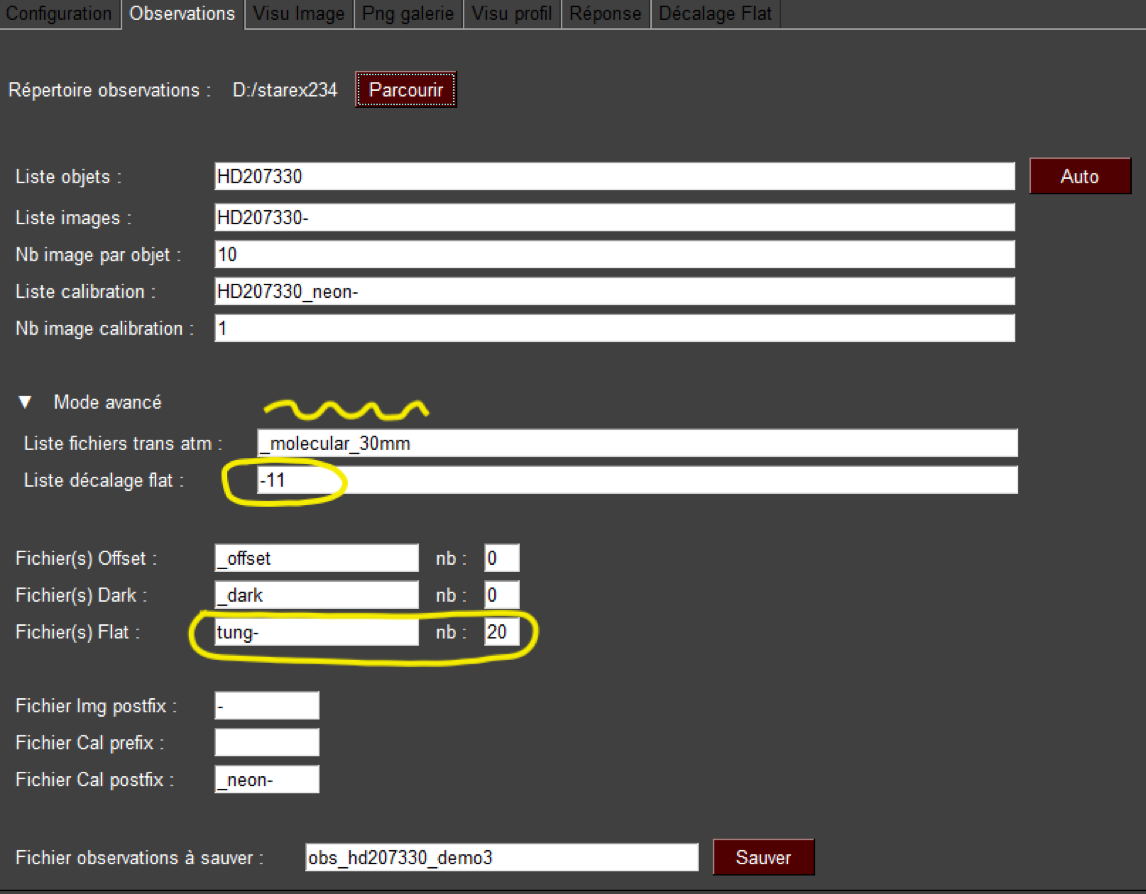
This is the way to indicate to specINTI that the flat-field made on the table must be shifted by -11 pixels before performing the division operation. Be careful, for the procedure to give a satisfactory result, it is imperative to indicate the list of raw images of the flat-field (generic name "tung-" and number of images equal to 20), and not the name of a reprocessed master flat-field ("_flat").
Don't worry, all these operations take longer to explain than to do, that's experience speaking!
Note: in the example we decided to correct the molecular atmospheric transmission, but note that this is an optional operation, which you can ignore to make your life easier.
Here is the appearance of the spectral profile of the star HD207330 with the application of the -11 pixel shift of the flat-field images and after the application of this shift :
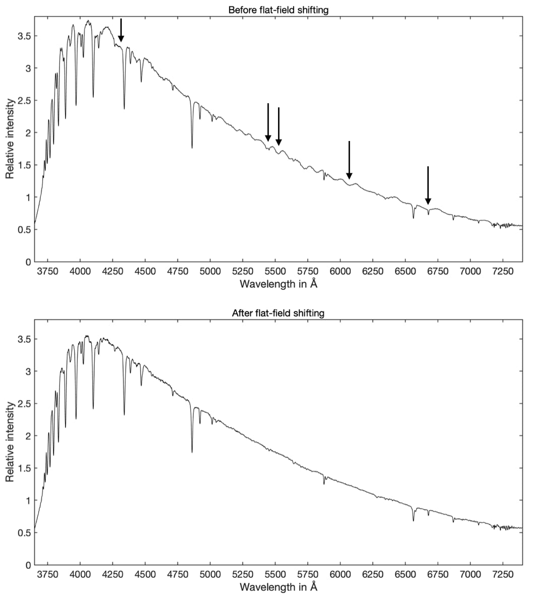
The parasitic fluctuations in the continuum have disappeared, and as a result the spectral profile thus treated is much closer to that expected for this type of star. In fact, thanks to our calculation artifice, the flat-field correction is almost perfect, despite the existence of quite severe mechanical bending. The flat-field did the job, despite the different conditions between the spectra taken at the telescope and the tungsten images on the table.
The exposed correction technique proves to be very reliable. For the record, it took several days between the moment when the observation on the sky was made and the moment when the flat-field was taken, and moreover the offset of -11 pixels is almost always the same on the Star'Ex we use (the value will surely be different for you, but probably constant, as long as you don't touch the orientation of the grating). This is so much so that we sometimes do not even measure the offset between observation and calibration on the table, trusting previous measurements!
9.9 : The evaluation of the instrumental response
The last step to finalize the treatment is the taking into account of the instrumental response (a true response, because our treatment has reduced the calculated spectrum to that seen from space). We recall the operation to be performed to find the instrumental response, that is to say the relative variation of sensitivity of the instrument (telescope + spectrograph + detector) as a function of the wavelength:
Instrumental response = (pre-processed apparent spectrum of a reference star) / (actual spectrum of the same reference star).
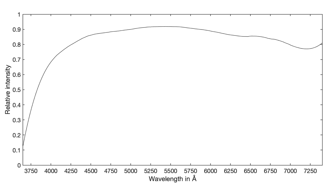
The choice of the star HD207330 is not trivial for this demonstration. It is a star whose real spectrum outside the atmosphere is known. It is a "reference" star, spectro-photometrically well calibrated. This spectrum can be found in the MILES spectral library (IAC), which is part of the ZIP archive downloaded in section 5.8.1. The spectrum in question is called "m_HD207330.fit" and here is its profile:
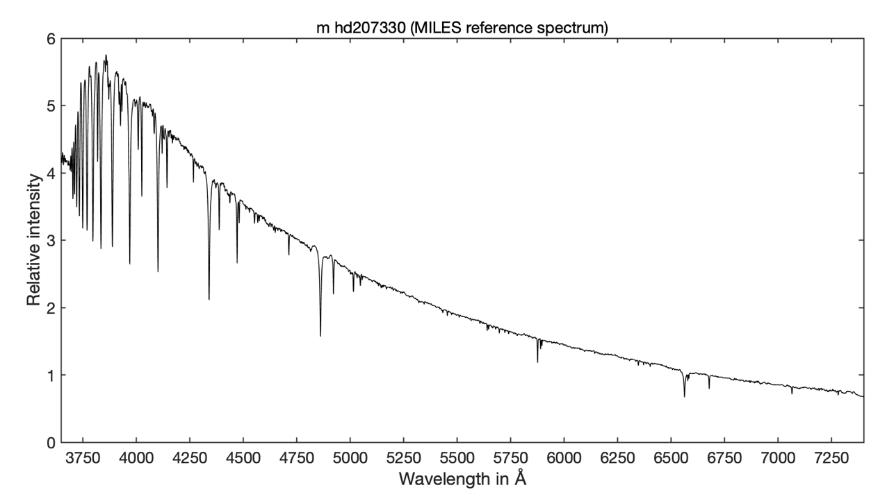
The division operation to find the instrumental response is unfortunately not immediately applicable, because the sharpness of our observed spectrum is lower than the MILES spectrum. A division as is will produce a large number of artifacts that will make it difficult to extract the effective response (with the low resolution Star'Ex as we use it, the resolving power is R=750-800, while it is about R=1400 for the MILES spectra).
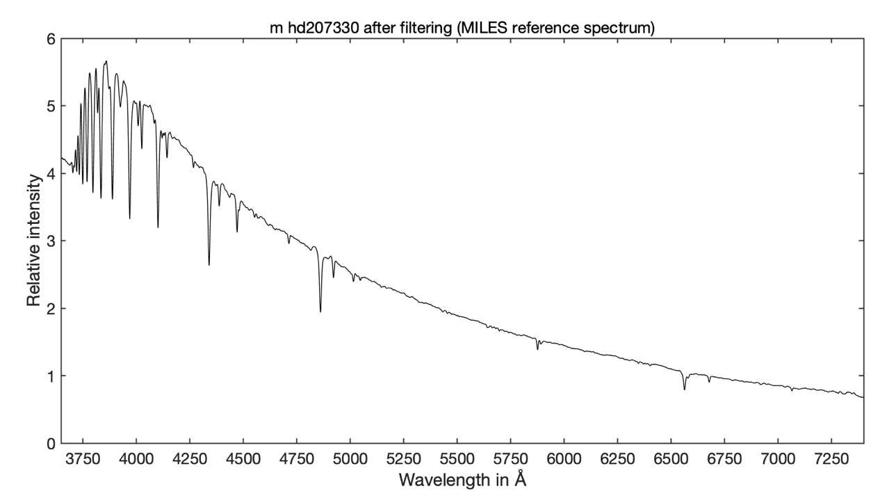
Before performing the division, we must therefore degrade the resolution of the spectrum "m_HD207330.fit". We will use the "_pro_gauss" function to do this. Insert this line in the configuration file, then run specINTI :
_pro_gauss: [_m_HD207330, 3, tempo1]
Note: the fact that the extension of this file is ".fit" when we have been working with files with the extension ".fits" is tolerated here. There will be no errors returned.
The _pro_gauss function performs a smoothing (or low-pass) filtering on the "m_HD270330" spectrum to produce the degraded resolution spectrum "tempo1".
The second parameter is the width of the smoothing function, which sets the strength of it. The stronger the value, the higher the action of the filter. In our case, we will choose the value 3,0 by experiment, to pass from a spectrum of R=1400 to R=800 (fractional values are taken into account, for example 3,5). You can make tests to see that the spectrum after smoothing resembles the spectrum observed. The smoothing coefficient thus established, by trial and error, will ultimately be a kind of constant for your instrument with respect to the MILES reference spectra. Here is the result after smoothing (spectrum "tempo1" in the example):
Delete the "_pro_gauss" line, or put a "#" in front of it so that it is considered a comment, then insert a new command:
_pro_div: [_hr207330_20220905_942, tempo1, tempo2]
As the name of this function suggests, it performs the operation:
tempo2 = _hr207330_20220905_942 / tempo1
We divide the spectrum found in the previous step (spectrum of the star without atmosphere and after division by the flat-field) by the theoretical spectrum of the star after smoothing. The result is the spectrum "tempo2", close to the true instrumental response sought:
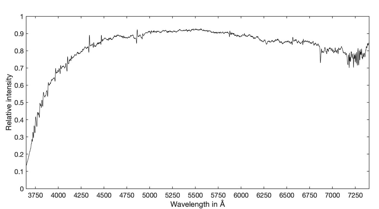
We observe in this result many roughnesses which do not need to be, coming from approximations of calculation and from deviations of modeling. An instrumental response curve worthy of the name is a monotonous, smooth curve. To erase these residual artifacts, we will perform a particular and energetic smoothing (SAVGOL algorithm), using a new function, "_pro_blur". As always, delete the line of the previous function and enter this new one:
_pro_blur: [tempo2, 1000, tempo3]
The tempo2 spectrum is the one to be cleaned of roughness. The parameter (1000) is a coefficient setting the strength of the filter, and tempo3 is the filtered spectrum. The value 1000 is typical of what should be done in this case, but you are perfectly entitled to test by rerunning the command with values 100, 2000, etc. Here is how the "demo3" spectrum looks:
To give a final touch, more aesthetic than anything else, and really optional, we can normalize the response in the same spectral range as the spectra of the sky objects:
_pro_norm: [tempo3, 6400, 6420, _rep]
The "_rep" file is the desired instrumental response!
Tip: in some rare situations, it is possible to launch several functions in a row by enclosing them with "_begin:" and "_end:" (don't forget the ":"). For example, for the calculation of the instrumental response :
_begin:
_pro_gauss: [_m_HD207330, 3, tempo1]
_pro_div: [_hr207330_20220905_942, tempo1, tempo2]
_pro_blur: [tempo2, 1000, tempo3]
_end:
And now, the good news: all these operations, which may seem heavy, manual, can be done graphically and immediately from the "Response" tab of the specINTI Editor interface:
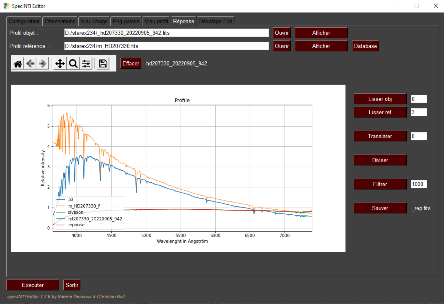
You will easily find the parameters used with the "functions" previously used: the names of the files at the top of the tab, then the level of smoothing of the reference spectrum (3.0) and the final filtering on the response (1000). At the end, you click on the "Save" button.
Another piece of good news is that the instrumental response file "_rep" is a constant, as we have often mentioned. You will very rarely have to do these operations again (and in theory never).
Somewhere in the configuration file, add the command "instrumental_response" so that the instrumental response is taken into account during processing. In our example, we simply write (the parameter value is the file name) :
instrumental_response: _rep
We now have everything we need to process the images of HD 207330 completely and extract the final spectrum. Here is how the "Observations" tab looks like for that:
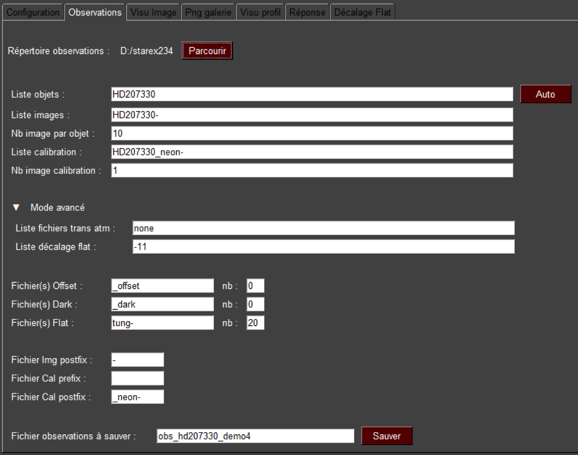
Note that we do not remove the telluric lines, seen here as effective details of the spectrum, even if they are parasites. Here is the associated configuration file, which you can copy/paste to process your own spectra (not only from a Star'Ex, but also from an Alpy600 or a LowSpec, which will be close in appearance and have the same requirements) :
# ********************************************************************
# Star'Ex low resolution configuration
# Calibration mode 2
# ********************************************************************
# ----------------------------------------------------------------
# Working directory
# ----------------------------------------------------------------
working_path: D:/starex234
# ----------------------------------------------------------------
# Processing batch file
# ----------------------------------------------------------------
batch_name: obs_hd207330_demo4
# ----------------------------------------------------------------
# Spectral calibration mode
# ----------------------------------------------------------------
calib_mode: 2
# ----------------------------------------------------------------
# Instrument response file name
# ----------------------------------------------------------------
instrumental_response: _rep
# -------------------------------------------------------------
# Coefficients of the calibration polynomial
# ------------------------------------------------------------
calib_coef: [1.008094181248435e-12, -4.8130567129843605e-09, 1.0804337072826731e-05, 1.5410557117037569, 3390.865801174948]
# -----------------------------------------------------------------------------
# Wavelength of the reference neon lines in A
# -----------------------------------------------------------------------------
wavelength: [5852.49, 6506.53]
# ----------------------------------------------------------------------------
# Position of the neon reference lines in pixels
# ----------------------------------------------------------------------------
line_pos: [1580, 2000]
# ---------------------------------------------------------------------------------------
# Width of the reference line search area
# ----------------------------------------------------------------------------------------
search_wide: 20
# ----------------------------------------------------------------
# Binning width
# ----------------------------------------------------------------
bin_size: 22
# ----------------------------------------------------------------
# Sky background calculation areas
# ----------------------------------------------------------------
sky: [120, 20, 20, 120]
# --------------------------------------------------------------------
# Color temperature of the tungsten lamp
# -------------------------------------------------------------------
planck: 2900
# ------------------------------------------------------------------
# Atmospheric transmission correction
# ------------------------------------------------------------------
corr_atmo: 0.13
# -------------------------------------------------------------------
# x-boundaries for geometric measurements
# ------------------------------------------------------------------
xlimit: [500, 2000]
# ----------------------------------------------------------------
# Normalization zone to the unit in A
# ----------------------------------------------------------------
norm_wave: [6400, 6420]
# ----------------------------------------------------------------
# Profile cropping area
# ----------------------------------------------------------------
crop_wave: [3700, 7400]
# ----------------------------------------------------------------
# Longitude of the observation place
# ----------------------------------------------------------------
Longitude: 7.0940
# ----------------------------------------------------------------
# Latitude of the observation site
# ----------------------------------------------------------------
Latitude: 43.5801
# ----------------------------------------------------------------
# Altitude of the observation point in meters
# ----------------------------------------------------------------
Altitude: 40
# ----------------------------------------------------------------
# Observation site
# ----------------------------------------------------------------
Site: Antibes Saint-Jean
# ----------------------------------------------------------------
# Description of the instrument
# ----------------------------------------------------------------
Inst: RC10 + StarEx300 + ASI533MM
# ----------------------------------------------------------------
# Observer
# ----------------------------------------------------------------
Observer: cbuil
# ------------------------------------------------------------------------
# FITS file extension (0 -> .fits, 1 - > fit)
# ------------------------------------------------------------------------
file_extension: 0
Le spectre final de HD207330 traité dans les règles, avec ce fichier de configuration :
Often, low resolution spectrography is aimed at studying objects with low brightness. Consider in this situation to activate the noise reduction tools, described in section 5.6. For example, add the following lines to your configuration file (file "conf_starex300_demo3.yaml" in the distribution):
# ---------------------------------------------------
# Sky extraction mode
# ---------------------------------------------------
sky_mode: 1
# ----------------------------------------------------------------
# Optimal extraction
# ----------------------------------------------------------------
extract_mode: 1
gain: 0.083
noise: 1.3
# ----------------------------------------------------------------
# Median filtering pattern
# 0: no filtering, otherwise: 3, 5, ...
# Negative value: optimized for impulse noise
# ----------------------------------------------------------------
kernel_size: -3
# ----------------------------------------------------------------
# Gaussian filtering
# ----------------------------------------------------------------
sigma_gauss: 0.4
9.10 : Serial processing
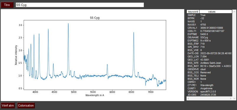
As you now know, without changing the configuration file, you can process anything your instrumentation generates (only the observation file changes, as well as its designation in the configuration file). For example, we will reduce both the spectra of HD 207330 and SS Cyg. For the latter object, the sequence is composed of 9 images of the spectrum and a neon lamp image made by illuminating the telescope entrance and taken at the end of the sequence. The object is of weak brilliance at the time of the observation, of magnitude 12 approximately, so that the exposure time adopted for each image is relatively long, 10 minutes (600 s). This remains however less than the basic time of the dark images (15 minutes).
Open the "Observations" tab and fill it in this way (remember to use the "Auto" button):
Remarquez que le champ « Liste décalage flat » est bien une liste comme le nom l’indique. Ainsi, vous pouvez entrer une translation différente du flat-field pour chaque série d’images à traiter, mais ici ce décalage est stable, donc la valeur reste -11 pour les deux astres traités. Lancez le traitement en cliquant sur « Exécuter », et au bout d’un moment :
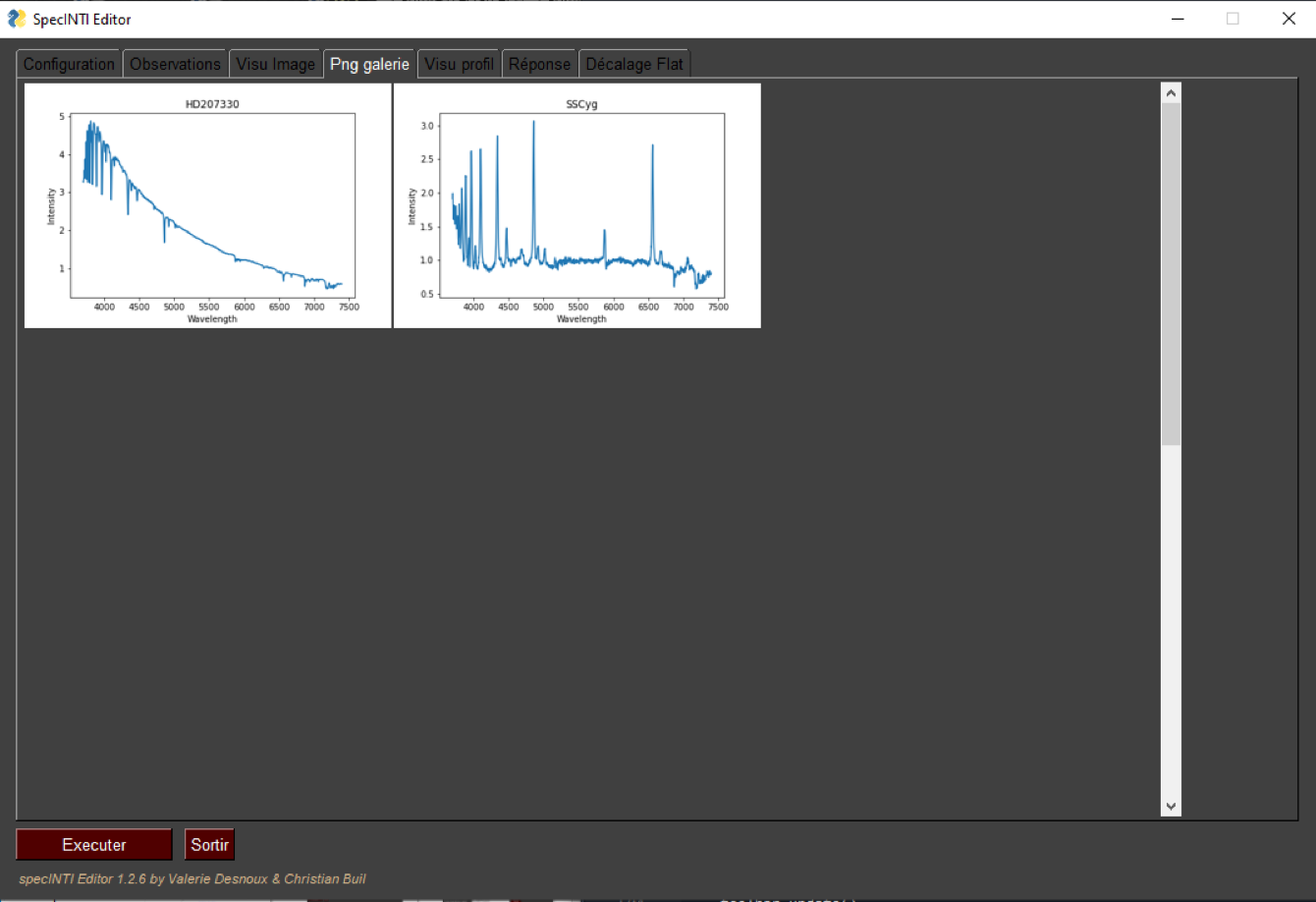
The spectrum of SS Cyg is characteristic of a symbiotic system "at rest" (we say in "quiescent" state), out of eruption. We see Balmer lines (hydrogen) as well as lines of helium in emission, but widened by the speed of gases (Doppler-Fizeau effect). The rise of the continuum at the beginning of the ultraviolet is real: